Maths
Statistics
Section titled “Statistics”Statistics is a branch of mathematics dealing with data collection, analysis, interpretation, and presentation. It provides tools for making informed decisions based on data.
Key Concepts
Section titled “Key Concepts”- Descriptive Statistics: Summarizes data using measures like mean, median, mode, and standard deviation.
- Inferential Statistics: Makes predictions or inferences about a population based on a sample of data.
Population vs Sample
Section titled “Population vs Sample”-
Population 📊
- Complete dataset
- Example: All students in a university
- N = Total size
-
Sample 🔍
- Subset of population
- Example: 100 randomly selected students
- n = Sample size
Key Point: Sample should be representative of the population
Measures of Central Tendency
Section titled “Measures of Central Tendency”-
Measures of Central Tendency are used to describe the central or typical value of a dataset.
-
Mean:
- Average of all values in a dataset
- Sample Formula: x̄ = (∑x) / n
- Population Formula: μ = (∑x) / N
- Example: For [2,4,6,8], Mean = (2+4+6+8)/4 = 5
- Use when:
- Data is normally distributed
- Need a value affected by all data points
- Limitations:
- Sensitive to outliers
- May not represent central value in skewed data
-
Median:
- Middle value when data is ordered
- Formula:
- Odd n: Value at position (n+1)/2
- Even n: Average of values at n/2 and (n/2)+1
- Example: For [1,3,5,7,9], Median = 5
- Use when:
- Data has outliers
- Distribution is skewed
- Limitations:
- Not influenced by all values
- Changes less smoothly than mean
-
Mode:
- Most frequently occurring value
- Formula: Value with highest frequency
- Example: For [1,2,2,3,4], Mode = 2
- Use when:
- Working with categorical data
- Need most common value
- Limitations:
- Can have multiple modes
- May not exist if all values occur once
Measures of Dispersion
Section titled “Measures of Dispersion”Measures of dispersion describe how spread out data points are from the center. They’re crucial for:
- Understanding data variability
- Assessing data reliability
- Comparing datasets
Common Measures
Section titled “Common Measures”-
Variance (σ²)
- Average squared deviation from mean
- Formula: σ² = Σ(x - μ)²/n
- Use when:
- Detailed spread analysis needed
- Computing statistical tests
- Limitation: Units are squared
-
Standard Deviation (σ)
- Square root of variance
- Formula: σ = √(Σ(x - μ)²/n)
- Use when:
- Need spread in original units
- Analyzing normal distributions
- Building ML models
Variance
Section titled “Variance”Variance measures the average squared distance of data points from their mean, indicating data spread and variability.
Key Points
Section titled “Key Points”- Definition: Average of squared deviations from mean
- Population Formula: σ² = Σ(x - μ)²/N
- Sample Formula: s² = Σ(x - x̄)²/(n-1)
Why Use n-1 in Sample Variance?
Section titled “Why Use n-1 in Sample Variance?”The use of (n-1) instead of n in sample variance is called Bessel’s Correction. Here’s why it matters:
-
Degrees of Freedom
- When calculating sample variance, we lose one degree of freedom
- This happens because we already used one piece of information (sample mean)
- n-1 accounts for this lost degree of freedom
-
Bias Correction
- Sample variance with n tends to underestimate population variance
- Using n-1 makes the estimator unbiased
- Formula: s² = Σ(x - x̄)²/(n-1)
-
Practical Impact
- More noticeable in small samples
- Example:
- n=5: 20% difference
- n=100: 1% difference
- Critical for accurate statistical inference
Real-World Example of n-1 in Sample Variance
Section titled “Real-World Example of n-1 in Sample Variance”Imagine a battery manufacturing plant:
Population Data:
- All 1000 batteries produced in a day
- True population mean (μ) = 1.5V
- Population readings vary between 1.3V to 1.7V
- True population variance = 0.024V²
Sample Test:
- We test only 5 batteries: [1.3V, 1.4V, 1.5V, 1.6V, 1.7V]
- Sample mean (x̄) = 1.5V
Variance Calculations:
# Using n (biased)Variance_n = Σ(x - x̄)²/5= [(1.3-1.5)² + (1.4-1.5)² + (1.5-1.5)² + (1.6-1.5)² + (1.7-1.5)²]/5= 0.02V² # Underestimates true variance (0.024V²)
# Using n-1 (unbiased)Variance_n1 = Σ(x - x̄)²/4= 0.025V² # Closer to true variance (0.024V²)
Why This Matters:
- Using n: 0.02V² (off by 0.004V²)
- Using n-1: 0.025V² (off by 0.001V²)
- n-1 gives estimate closer to true population variance
This example shows how n-1 provides a better estimate of the true population variance. Note that in real situations, we usually don’t know the true population variance - that’s why we need good estimation methods.
Key Point: Use n-1 for sample variance to get an unbiased estimate of population variance
# Sample of 100 people's weightsmean = 70kgvariance = 25kg²  # Standard deviation ≈ 5kg
# Practical Usesize_range = mean ± (2 × √variance)# = 70 ± 10kg# = 60kg to 80kg
# Example with weight datamean = 70kgstd_dev = 5kg
# Coverage ranges1σ range = 70 ± 5kg   = 65-75kg   (covers 68%)2σ range = 70 ± 10kg  = 60-80kg   (covers 95%)  # Most commonly used3σ range = 70 ± 15kg  = 55-85kg   (covers 99.7%)
Variables
Section titled “Variables”Variables are characteristics that can be measured or categorized. They come in different types:
1. Qualitative (Categorical) Variables
Section titled “1. Qualitative (Categorical) Variables”-
Nominal
- Categories with no order
- Example: Colors (red, blue), Gender (male, female)
- Analysis: Mode, frequency
-
Ordinal
- Categories with order
- Example: Education (high school, bachelor’s, master’s)
- Analysis: Median, percentiles
2. Quantitative (Numerical) Variables
Section titled “2. Quantitative (Numerical) Variables”-
Discrete
- Countable values
- Example: Number of children, Test score
- Analysis: Mean, standard deviation
-
Continuous
- Infinite possible values
- Example: Height, Weight, Time
- Analysis: Mean, standard deviation, correlation
Variable Relationships
Section titled “Variable Relationships”-
Independent Variable (X)
- Manipulated/controlled variable
- Example: Study hours
-
Dependent Variable (Y)
- Outcome variable
- Example: Test score
Note: Variable type determines which statistical methods to use
Random Variables
Section titled “Random Variables”A random variable is a function that assigns numerical values to outcomes of a random experiment.
Types of Random Variables
Section titled “Types of Random Variables”-
Discrete Random Variables
- Takes countable/finite values
- Examples:
- Number of heads in coin flips
- Count of defective items
- Properties:
- Probability Mass Function (PMF)
- Cumulative Distribution Function (CDF)
-
Continuous Random Variables
- Takes infinite possible values
- Examples:
- Height of a person
- Time to complete a task
- Properties:
- Probability Density Function (PDF)
- Cumulative Distribution Function (CDF)
Histogram
Section titled “Histogram”A histogram is a graphical representation of the distribution of data. It shows the frequency of each data point in a dataset.
Key Points
Section titled “Key Points”- Definition: Bar chart showing frequency of data points
- Purpose: Visualize data distribution
- Components:
- X-axis: Data range (bins)
- Y-axis: Frequency (count or percentage)
- Bars: Represents frequency of data in each bin
Examples
Section titled “Examples”import numpy as npimport matplotlib.pyplot as plt
data = [1, 2, 2, 3, 3, 3, 4, 4, 5]plt.figure(figsize=(8, 4))plt.hist(data, bins=5, edgecolor='black')plt.title('Simple Histogram')plt.xlabel('Values')plt.ylabel('Frequency')plt.show()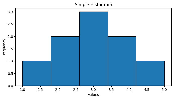
Percentiles and Quartiles
Section titled “Percentiles and Quartiles”Percentiles and quartiles are measures that divide a dataset into equal portions.
Percentiles
Section titled “Percentiles”- Divides data into 100 equal parts
- Pth percentile: Value below which P% of observations fall
- Common uses:
- 50th percentile = median
- Used in standardized testing (e.g., “90th percentile”)
Quartiles
Section titled “Quartiles”- Divides data into 4 equal parts
- Q1 (25th percentile): First quartile
- Q2 (50th percentile): Median
- Q3 (75th percentile): Third quartile
- IQR (Interquartile Range) = Q3 - Q1
Example
Section titled “Example”import numpy as np
data = [2, 4, 6, 8, 10, 12, 14, 16]
# QuartilesQ1 = np.percentile(data, 25) # = 5Q2 = np.percentile(data, 50) # = 9Q3 = np.percentile(data, 75) # = 13IQR = Q3 - Q1 # = 8
# Any percentilep90 = np.percentile(data, 90) # 14.65 Number Summary
Section titled “5 Number Summary”The 5 number summary is a quick way to describe the distribution of a dataset. It consists of the minimum, first quartile, median, third quartile, and maximum.
- Minimum: Smallest value in the dataset
- First Quartile (Q1): 25th percentile
- Median: 50th percentile
- Third Quartile (Q3): 75th percentile
- Maximum: Largest value in the dataset
Example
Section titled “Example”import numpy as np
data = [2, 4, 6, 8, 10, 12, 14, 16]
# 5 Number Summarysummary = np.percentile(data, [0, 25, 50, 75, 100])print(summary) # [2. 5. 9. 13. 16.]Outliers are values that fall outside the range of the 5 number summary.
- Lower Outlier: Below (Q1 - 1.5 * IQR)
- Upper Outlier: Above (Q3 + 1.5 * IQR)
- Interquartile Range (IQR) = Q3 - Q1
Example
Section titled “Example”import numpy as np
# Sample datasetdata = [1, 2, 2, 3, 4, 10, 20, 25, 30]
# Calculate 5 number summarymin_val = np.min(data)q1 = np.percentile(data, 25)median = np.percentile(data, 50)q3 = np.percentile(data, 75)max_val = np.max(data)
# Calculate IQR and outlier boundsiqr = q3 - q1lower_bound = q1 - 1.5 * iqrupper_bound = q3 + 1.5 * iqr
# Find outliersoutliers = [x for x in data if x < lower_bound or x > upper_bound]
print(f"5 Number Summary:")print(f"Min: {min_val}")print(f"Q1: {q1}")print(f"Median: {median}")print(f"Q3: {q3}")print(f"Max: {max_val}")print(f"Outliers: {outliers}")Covariance and Correlation
Section titled “Covariance and Correlation”Covariance
Section titled “Covariance”Covariance measures how two variables change together. It indicates the direction of the linear relationship between variables.
Formula
Section titled “Formula”- Population Covariance: σxy = Σ((x - μx)(y - μy))/N
- Sample Covariance: sxy = Σ((x - x̄)(y - ȳ))/(n-1)
Interpretation
Section titled “Interpretation”- Positive covariance: Variables tend to move in same direction
- Negative covariance: Variables tend to move in opposite directions
- Zero covariance: No linear relationship
Example
Section titled “Example”import numpy as np
# Height (cm) and Weight (kg) dataheight = np.array([170, 175, 160, 180, 165, 172])weight = np.array([65, 70, 55, 80, 60, 68])
# Calculate meansheight_mean = np.mean(height)weight_mean = np.mean(weight)
# Calculate covariance manuallyn = len(height)covariance = sum((height - height_mean) * (weight - weight_mean)) / (n-1)
# Using NumPycov_matrix = np.cov(height, weight)covariance_np = cov_matrix[0,1]
print(f"Manual Covariance: {covariance:.2f}")print(f"NumPy Covariance: {covariance_np:.2f}")
# Output:# Manual Covariance: 58.17# NumPy Covariance: 58.17Key Points:
Section titled “Key Points:”- Covariance range: -∞ to +∞
- Scale-dependent (affected by units)
- Used in:
- Principal Component Analysis
- Portfolio optimization
- Feature selection in ML
Limitations:
Section titled “Limitations:”- Not standardized (hard to compare)
- Units are product of both variables
For standardized measurement, use correlation instead.
Correlation
Section titled “Correlation”Correlation measures the strength and direction of the linear relationship between two variables. Unlike covariance, it’s standardized between -1 and +1.
Pearson Correlation Coefficient
Section titled “Pearson Correlation Coefficient”The most common correlation measure is Pearson’s r:
Formula
Section titled “Formula”- Population Correlation: ρxy = Σ((x - μx)(y - μy))/(σxσy)
- Sample Correlation: r = Σ((x - x̄)(y - ȳ))/√[Σ(x - x̄)²Σ(y - ȳ)²] = Cov(x,y)/(σxσy)
Interpretation
Section titled “Interpretation”- r = 1: Perfect positive correlation
- r = -1: Perfect negative correlation
- r = 0: No linear correlation
- |r| > 0.7: Strong correlation
- 0.3 < |r| < 0.7: Moderate correlation
- |r| < 0.3: Weak correlation
Example
Section titled “Example”import numpy as npimport matplotlib.pyplot as plt
# Sample datax = np.array([1, 2, 3, 4, 5])y1 = np.array([2, 4, 6, 8, 10]) # Perfect positivey2 = np.array([10, 8, 6, 4, 2]) # Perfect negativey3 = np.array([2, 5, 4, 5, 3]) # Weak correlation
def plot_correlation(x, y, title): plt.scatter(x, y) plt.title(f'{title} (r = {np.corrcoef(x,y)[0,1]:.2f})') plt.xlabel('X') plt.ylabel('Y')
# Create subplotsplt.figure(figsize=(15, 5))
plt.subplot(131)plot_correlation(x, y1, "Perfect Positive")
plt.subplot(132)plot_correlation(x, y2, "Perfect Negative")
plt.subplot(133)plot_correlation(x, y3, "Weak")
plt.tight_layout()plt.show()
# Calculate correlationsprint(f"Positive correlation: {np.corrcoef(x,y1)[0,1]:.2f}") # 1.00print(f"Negative correlation: {np.corrcoef(x,y2)[0,1]:.2f}") # -1.00print(f"Weak correlation: {np.corrcoef(x,y3)[0,1]:.2f}") # 0.24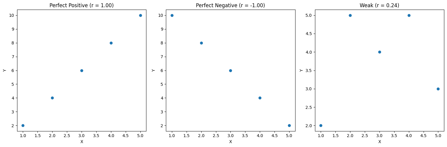
Key Properties
Section titled “Key Properties”- Scale-independent (standardized)
- Always between -1 and +1
- No units
- Symmetric: corr(x,y) = corr(y,x)
Common Uses
Section titled “Common Uses”- Feature selection in ML
- Financial portfolio analysis
- Scientific research
- Quality control
Limitations
Section titled “Limitations”- Only measures linear relationships
- Sensitive to outliers
- Correlation ≠ causation
- Requires numeric data
Real-World Example
Section titled “Real-World Example”import pandas as pd
# Student datadata = { 'study_hours': [2, 3, 3, 4, 4, 5, 5, 6], 'test_score': [65, 70, 75, 80, 85, 85, 90, 95]}
df = pd.DataFrame(data)
# Calculate correlationcorrelation = df['study_hours'].corr(df['test_score'])
print(f"Correlation between study hours and test scores: {correlation:.2f}")# Output: Correlation between study hours and test scores: 0.97Important Notes
Section titled “Important Notes”- High correlation doesn’t imply causation
- Always visualize data - don’t rely solely on correlation coefficient
- Consider non-linear relationships
- Check for outliers that might affect correlation
Spearman Correlation
Section titled “Spearman Correlation”Spearman correlation measures monotonic relationships between variables (whether they move in the same direction, regardless of the rate of change).
Formula
Section titled “Formula”-
First convert values to ranks
- rank(x): Rank values of first variable
- rank(y): Rank values of second variable
-
Calculate differences d = rank(x) - rank(y)
-
Square the differences d² = (rank(x) - rank(y))²
-
Sum all squared differences Σd² = sum of all d²
-
Final formula: ρ = 1 - (6 * Σd²)/(n(n² - 1))
Example with numbers: x = [1,2,3] y = [2,1,3]
ranks_x = [1,2,3] ranks_y = [2,1,3]
d = [1-2, 2-1, 3-3] = [-1,1,0] d² = [1,1,0] Σd² = 2 n = 3
ρ = 1 - (6 * 2)/(3(9-1)) = 1 - 12/24 = 0.5
Example
Section titled “Example”import numpy as npimport matplotlib.pyplot as pltfrom scipy import stats
# Online Store Example# X: Product Price# Y: Number of Salesprice = np.array([10, 20, 30, 40, 50, 60, 70, 80, 90, 100])sales = np.array([100, 90, 80, 65, 45, 30, 20, 15, 12, 10])
# Calculate Correlationspearson = stats.pearsonr(price, sales)[0]spearman = stats.spearmanr(price, sales)[0]
# Plottingplt.figure(figsize=(10, 6))plt.scatter(price, sales)plt.title('Price vs Sales: Non-linear Relationship')plt.xlabel('Price ($)')plt.ylabel('Number of Sales')
# Add correlation valuesplt.text(20, 30, f'Pearson r: {pearson:.2f}')plt.text(20, 20, f'Spearman r: {spearman:.2f}')plt.grid(True)plt.show()
print(f"Pearson Correlation: {pearson:.2f}") # -0.89print(f"Spearman Correlation: {spearman:.2f}") # -1.00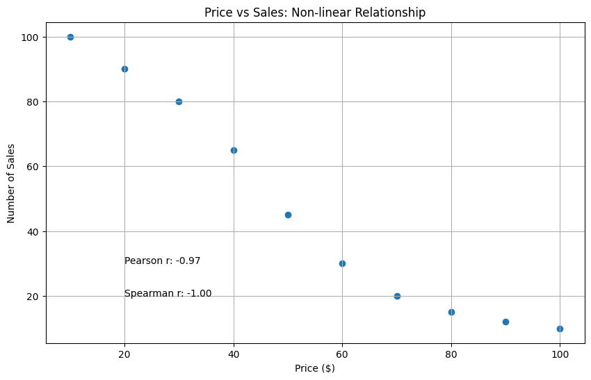
Probability
Section titled “Probability”Probability is a measure of the likelihood of an event occurring. It’s a fundamental concept in statistics and data science.
Additive Rule
Section titled “Additive Rule”Mutually Exclusive Events
Section titled “Mutually Exclusive Events”Events that cannot occur at the same time.
Formula: P(A or B) = P(A) + P(B)
Example:
- Rolling a die:
- P(getting 1 or 2) = P(1) + P(2) = 1/6 + 1/6 = 1/3
- Events are mutually exclusive since you can’t roll 1 and 2 simultaneously
Non-Mutually Exclusive Events
Section titled “Non-Mutually Exclusive Events”Events that can occur at the same time.
Formula: P(A or B) = P(A) + P(B) - P(A and B)
Example:
- Drawing a card:
- P(getting King or Heart) = P(King) + P(Heart) - P(King of Heart)
- = 4/52 + 13/52 - 1/52 = 16/52
- Events overlap since King of Hearts is possible
Multiplicative Rule
Section titled “Multiplicative Rule”The multiplicative rule calculates probability of multiple events occurring together.
Independent Events
Section titled “Independent Events”Events where occurrence of one doesn’t affect the other.
Formula: P(A and B) = P(A) × P(B)
Example:
- Flipping a coin twice:
- P(2 heads) = P(head1) × P(head2) = 1/2 × 1/2 = 1/4
Dependent Events
Section titled “Dependent Events”Events where occurrence of one affects the other.
Formula: P(A and B) = P(A) × P(B|A)
Example:
- Drawing 2 cards without replacement:
- P(2 aces) = P(ace1) × P(ace2|ace1)
- = 4/52 × 3/51 = 1/221
Relationship between PMF, PDF, and CDF
Section titled “Relationship between PMF, PDF, and CDF”1. PMF (Probability Mass Function)
Section titled “1. PMF (Probability Mass Function)”A PMF describes the probability distribution of a discrete random variable.
Definition
Section titled “Definition”- Maps each value of discrete random variable to its probability
- P(X = x) gives probability of X taking value x
- Sum of all probabilities must equal 1
Properties
Section titled “Properties”- 0 ≤ P(X = x) ≤ 1
- ∑P(X = x) = 1
- Only for discrete variables
Real-World Example: Dice Roll Game
Section titled “Real-World Example: Dice Roll Game”import numpy as npimport matplotlib.pyplot as plt
# Fair die PMFoutcomes = np.array([1, 2, 3, 4, 5, 6])probabilities = np.array([1/6] * 6)
# Loaded die PMF (favors 6)loaded_prob = np.array([0.1, 0.1, 0.1, 0.1, 0.1, 0.5])
# Plotplt.figure(figsize=(10, 5))plt.subplot(1, 2, 1)plt.bar(outcomes, probabilities)plt.title('Fair Die PMF')plt.xlabel('Outcome')plt.ylabel('Probability')
plt.subplot(1, 2, 2)plt.bar(outcomes, loaded_prob)plt.title('Loaded Die PMF')plt.xlabel('Outcome')plt.show()
# Calculate probability of rolling even numbersfair_even = sum(probabilities[1::2]) # 0.5loaded_even = sum(loaded_prob[1::2]) # 0.7
print(f"P(Even) Fair Die: {fair_even}") # 0.5print(f"P(Even) Loaded Die: {loaded_even}") # 0.7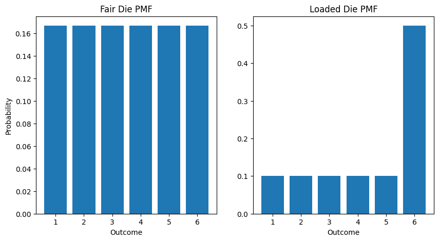
PMF helps in making probability-based decisions in discrete scenarios like manufacturing defects, customer counts, or game outcomes.
CDF (Cumulative Distribution Function) For Discrete Variables
Section titled “CDF (Cumulative Distribution Function) For Discrete Variables”CDF gives the probability that a random variable X is less than or equal to a value x.
Formula
Section titled “Formula”F(x) = P(X ≤ x) = ∑ P(X = t) for all t ≤ x
Example: Die Roll
Section titled “Example: Die Roll”import numpy as npimport matplotlib.pyplot as plt
# Define probabilitiesoutcomes = np.arange(1, 7) # [1,2,3,4,5,6]fair_prob = np.ones(6) / 6 # [1/6, 1/6, 1/6, 1/6, 1/6, 1/6]loaded_prob = np.array([0.1, 0.1, 0.1, 0.1, 0.1, 0.5])
# Calculate CDFsfair_cdf = np.cumsum(fair_prob)loaded_cdf = np.cumsum(loaded_prob)
# Create plotfig, (ax1, ax2) = plt.subplots(1, 2, figsize=(10, 5))
# Plot fair die CDFax1.step(outcomes, fair_cdf, where='post')ax1.set(title='Fair Die CDF', xlabel='Outcome', ylabel='Cumulative Probability')ax1.grid(True)
# Plot loaded die CDFax2.step(outcomes, loaded_cdf, where='post')ax2.set(title='Loaded Die CDF', xlabel='Outcome')ax2.grid(True)
plt.tight_layout()plt.show()
# Print probabilities for X ≤ 4print(f"P(X ≤ 4) Fair Die: {fair_cdf[3]:.3f}") # 0.667print(f"P(X ≤ 4) Loaded Die: {loaded_cdf[3]:.3f}") # 0.400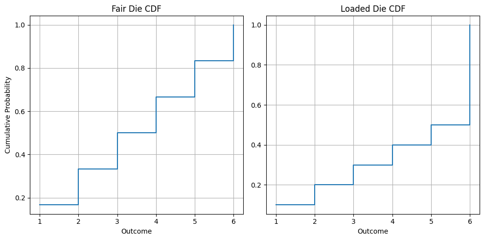
2. PDF (Probability Density Function)
Section titled “2. PDF (Probability Density Function)”A PDF describes the probability distribution of a continuous random variable.
Why PDF for Continuous Random Variables?
Section titled “Why PDF for Continuous Random Variables?”-
Impossible to List All Values
- Continuous variables have infinite possible values
- Can’t assign individual probabilities like PMF
-
Zero Individual Probability
- P(X = x) = 0 for any exact value
- Example: P(height = exactly 170.000000…cm) = 0
-
Range Probabilities
- PDF helps calculate probability over intervals
- P(a ≤ X ≤ b) = ∫[a to b] f(x)dx
- Example: P(170 ≤ height ≤ 175)
import numpy as npimport matplotlib.pyplot as pltfrom scipy.stats import norm
# Height Distribution in Adult Populationmean_height = 170  # cmstd_dev = 10       # cm
# Create height rangeheights = np.linspace(140, 200, 100)
# Calculate PDF using normal distributionpdf = norm.pdf(heights, mean_height, std_dev)
# Plotplt.figure(figsize=(10, 6))plt.plot(heights, pdf)plt.title('Height Distribution in Adult Population')plt.xlabel('Height (cm)')plt.ylabel('Probability Density')
# Calculate probabilities# Probability of height between 160-180cmprob_160_180 = norm.cdf(180, mean_height, std_dev) - norm.cdf(160, mean_height, std_dev)print(f"Probability of height between 160-180cm: {prob_160_180:.2%}")  # ≈ 68%
# Probability of height above 190cmprob_above_190 = 1 - norm.cdf(190, mean_height, std_dev)print(f"Probability of height above 190cm: {prob_above_190:.2%}")      # ≈ 2.3%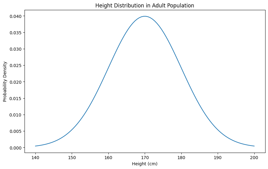
Density
Section titled “Density”Density in statistics refers to how tightly packed data points or probability is in a given interval or region.
import numpy as npfrom scipy.stats import normimport matplotlib.pyplot as plt
mean = 170std = 10
# Single point density doesn't tell muchpoint_density = norm.pdf(170, mean, std)print(f"Density at 170cm: {point_density:.4f}")  # 0.0399# This number 0.0399 alone is meaningless without context
# What makes sense is comparing densitiesheights = [150, 160, 170, 180, 190]densities = [norm.pdf(h, mean, std) for h in heights]
plt.figure(figsize=(10, 6))x = np.linspace(140, 200, 1000)y = norm.pdf(x, mean, std)
plt.plot(x, y)
# Plot points for comparisonfor h, d in zip(heights, densities):    plt.plot(h, d, 'o', label=f'Height={h}cm\nDensity={d:.4f}')
plt.title('Height Distribution - Comparing Densities')plt.xlabel('Height (cm)')plt.ylabel('Density')plt.legend()plt.grid(True)
# Now we can see:# - 170cm has highest density (most common)# - 150cm and 190cm have low density (less common)# - Comparison gives meaning to the numbers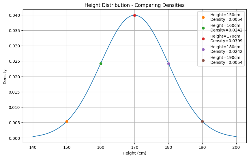
CDF (Cumulative Distribution Function) For Continuous Variables
Section titled “CDF (Cumulative Distribution Function) For Continuous Variables”The Cumulative Distribution Function (CDF) for a continuous random variable X, denoted as F(x), represents the probability that X takes on a value less than or equal to x.
Mathematical Definition
Section titled “Mathematical Definition”F(x) = P(X ≤ x) = ∫[from -∞ to x] f(t)dt
where f(t) is the probability density function (PDF)
Key Properties
Section titled “Key Properties”-
Bounds
- 0 ≤ F(x) ≤ 1 for all x
- lim[x→-∞] F(x) = 0
- lim[x→∞] F(x) = 1
-
Continuity
- Right-continuous
- Monotonically increasing (never decreases)
-
Probability Calculations
- P(a < X ≤ b) = F(b) - F(a)
- P(X > a) = 1 - F(a)
-
Relationship to PDF
- F’(x) = f(x) (derivative of CDF is PDF)
- F(x) is the integral of f(x)
Simple Example: Height Distribution in a Class
Section titled “Simple Example: Height Distribution in a Class”Consider heights of students in a class of 100:
Scenario:
- Heights range from 150cm to 190cm
- CDF tells us probability of height being less than or equal to a value
Simple Interpretations:
- F(160) = 0.2 means 20% of students are 160cm or shorter
- F(170) = 0.5 means 50% of students are 170cm or shorter
- F(180) = 0.9 means 90% of students are 180cm or shorter
Practical Uses:
- Finding median height: Where F(x) = 0.5
- Ordering uniforms: What size covers 80% of students
- Identifying unusually tall/short: Heights where F(x) < 0.1 or F(x) > 0.9
import numpy as npimport matplotlib.pyplot as pltfrom scipy.stats import norm
# Parametersmean_height = 170  # mean height in cmstd_dev = 10      # standard deviation in cmn_students = 100
# Generate student heightsnp.random.seed(42)  # for reproducibilityheights = np.random.normal(mean_height, std_dev, n_students)
# Calculate empirical CDFheights_sorted = np.sort(heights)cumulative_prob = np.arange(1, len(heights) + 1) / len(heights)
# Plotplt.figure(figsize=(10, 6))
# Empirical CDFplt.plot(heights_sorted, cumulative_prob, 'b-', label='Empirical CDF')
# Add reference linesplt.axhline(y=0.2, color='r', linestyle='--', alpha=0.5)plt.axhline(y=0.5, color='r', linestyle='--', alpha=0.5)plt.axhline(y=0.9, color='r', linestyle='--', alpha=0.5)
# Labels and titleplt.title('Height Distribution CDF in Class')plt.xlabel('Height (cm)')plt.ylabel('Cumulative Probability')plt.grid(True)
# Find specific valuesheight_20 = np.percentile(heights, 20)height_50 = np.percentile(heights, 50)height_90 = np.percentile(heights, 90)
print(f"20th percentile (F(x) = 0.2): {height_20:.1f}cm") # 162.6cmprint(f"50th percentile (F(x) = 0.5): {height_50:.1f}cm") # 168.7cmprint(f"90th percentile (F(x) = 0.9): {height_90:.1f}cm") # 180.1cm
plt.show()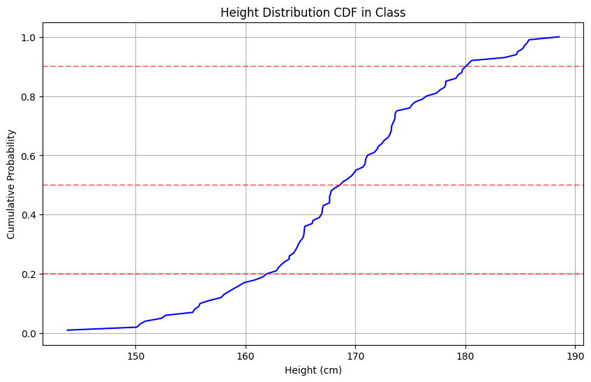
Types of Probability Distributions
Section titled “Types of Probability Distributions”Bernoulli Distribution
Section titled “Bernoulli Distribution”The Bernoulli distribution models binary outcomes - experiments with exactly two possible results (success/failure).
Properties
Section titled “Properties”- Parameter: p (probability of success)
- Possible Values: x ∈ 1
- x = 1 (success): probability = p
- x = 0 (failure): probability = 1-p
- PMF: P(X = x) = p^x * (1-p)^(1-x)
- Mean: E(X) = p
- Variance: Var(X) = p(1-p)
Common Applications
Section titled “Common Applications”- Coin flips (heads/tails)
- Quality control (defective/non-defective)
- Email (spam/not spam)
- Medical tests (positive/negative)
Example Implementation
Section titled “Example Implementation”import numpy as npimport matplotlib.pyplot as plt
class BernoulliTrial: def __init__(self, p): self.p = p
def pmf(self, x): return self.p if x == 1 else (1-self.p)
def simulate(self, n_trials): return np.random.binomial(n=1, p=self.p, size=n_trials)
# Example: Biased coin (p=0.7)b = BernoulliTrial(p=0.7)trials = b.simulate(1000)
# Resultssuccess_rate = np.mean(trials)print(f"Theoretical probability: 0.7")print(f"Observed probability: {success_rate:.3f}")
# Visualizeplt.figure(figsize=(8, 4))plt.bar(['Failure (0)', 'Success (1)'], [1-success_rate, success_rate])plt.title('Bernoulli Distribution (p=0.7)')plt.ylabel('Probability')plt.ylim(0, 1)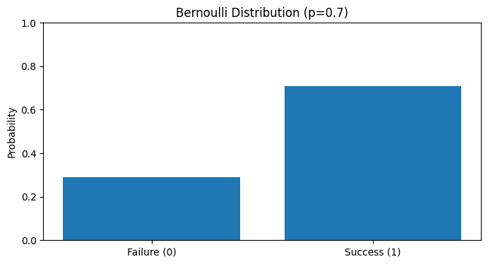
Real-World Example: Email Spam Detection
Section titled “Real-World Example: Email Spam Detection”# Simple spam detectorclass SpamDetector: def __init__(self, spam_probability=0.3): self.b = BernoulliTrial(spam_probability)
def classify_email(self): return "Spam" if self.b.simulate(1)[0] else "Not Spam"
# Simulate email classificationdetector = SpamDetector()n_emails = 100classifications = [detector.classify_email() for _ in range(n_emails)]
spam_ratio = classifications.count("Spam") / n_emailsprint(f"Classified {spam_ratio:.1%} emails as spam")// Classified 26.0% emails as spamKey Points
Section titled “Key Points”- Independence: Each trial is independent
- Memory-less: Previous outcomes don’t affect next trial
- Fixed probability: p remains constant across trials
Relationship to Other Distributions
Section titled “Relationship to Other Distributions”- Foundation for Binomial distribution (n Bernoulli trials)
- Special case of Binomial where n=1
- Building block for more complex probability models
Binomial Distribution
Section titled “Binomial Distribution”The Binomial distribution models the number of successes in n independent Bernoulli trials.
Properties
Section titled “Properties”- Parameters:
- n (number of trials)
- p (probability of success)
- PMF: P(X = k) = C(n,k) * p^k * (1-p)^(n-k)
- Mean: E(X) = np
- Variance: Var(X) = np(1-p)
Example Implementation
Section titled “Example Implementation”import numpy as npimport matplotlib.pyplot as pltfrom scipy.stats import binom
class BinomialDistribution: def __init__(self, n, p): self.n = n self.p = p
def pmf(self, k): return binom.pmf(k, self.n, self.p)
def simulate(self, n_trials): return np.random.binomial(self.n, self.p, n_trials)
# Example: Rolling a fair die 10 times, counting 6sn, p = 10, 1/6 # 10 rolls, P(6) = 1/6b = BinomialDistribution(n, p)
# Calculate PMF for all possible valuesk = np.arange(0, n+1)probabilities = [b.pmf(ki) for ki in k]
# Plotplt.figure(figsize=(10, 5))plt.bar(k, probabilities)plt.title(f'Binomial Distribution (n={n}, p={p:.2f})')plt.xlabel('Number of Successes (k)')plt.ylabel('Probability')plt.grid(True, alpha=0.3)
# Expected value and variancemean = n * pvar = n * p * (1-p)print(f"Expected number of 6s: {mean:.2f}") # 1.67print(f"Variance: {var:.2f}") # 1.39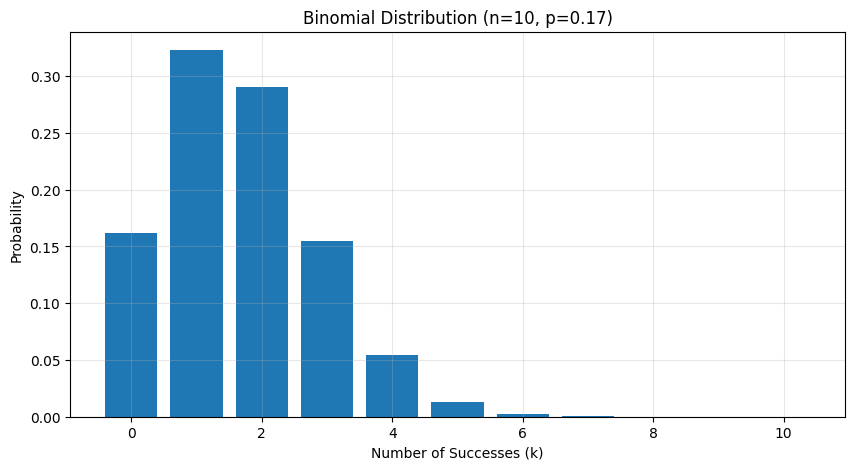
Real-World Example: Quality Control
Section titled “Real-World Example: Quality Control”# Manufacturing defect inspectionclass QualityControl: def __init__(self, batch_size=20, defect_rate=0.05): self.binom = BinomialDistribution(batch_size, defect_rate)
def inspect_batch(self): return self.binom.simulate(1)[0]
def is_batch_acceptable(self, max_defects=2): defects = self.inspect_batch() return { 'defects': defects, 'acceptable': defects <= max_defects }
# Simulate batch inspectionsqc = QualityControl()n_batches = 1000inspections = [qc.is_batch_acceptable() for _ in range(n_batches)]
acceptance_rate = sum(i['acceptable'] for i in inspections) / n_batchesprint(f"Batch acceptance rate: {acceptance_rate:.1%}")// Batch acceptance rate: 92.7%Common Applications
Section titled “Common Applications”- Quality control in manufacturing
- A/B testing success counts
- Survey response modeling
- Genetic inheritance patterns
Key Points
Section titled “Key Points”- Sum of independent Bernoulli trials
- Requires fixed probability p
- Trials must be independent
- Only whole numbers (discrete)
Poisson Distribution
Section titled “Poisson Distribution”The Poisson distribution models the number of events occurring in a fixed interval when these events happen at a constant average rate and independently of each other.
Properties
Section titled “Properties”- Parameter: λ (lambda) - average number of events per interval
- PMF: P(X = k) = (λ^k * e^-λ) / k!
- Mean: E(X) = λ
- Variance: Var(X) = λ
import numpy as npimport matplotlib.pyplot as pltfrom scipy.stats import poisson
class PoissonDistribution:    def __init__(self, lambda_param):        self.lambda_param = lambda_param
    def pmf(self, k):        return poisson.pmf(k, self.lambda_param)
    def simulate(self, n_samples):        return np.random.poisson(self.lambda_param, n_samples)
# Example: Website visits per hour (average 5 visits)lambda_param = 5p = PoissonDistribution(lambda_param)
# Calculate PMF for values 0 to 12k = np.arange(0, 13)probabilities = [p.pmf(ki) for ki in k]
# Visualizationplt.figure(figsize=(10, 6))plt.bar(k, probabilities)plt.title(f'Poisson Distribution (λ={lambda_param})')plt.xlabel('Number of Events (k)')plt.ylabel('Probability')plt.grid(True, alpha=0.3)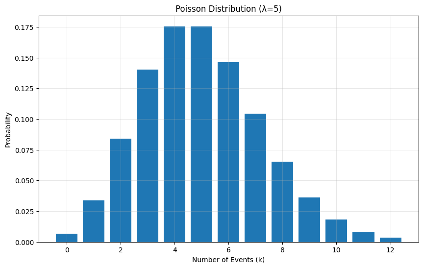
Common Applications
Section titled “Common Applications”-
Customer Service
- Number of customers arriving per hour
- Support tickets received per day
- Phone calls to call center
-
Web Traffic
- Page views per minute
- Server requests per second
- Error occurrences per day
-
Quality Control
- Defects per unit area
- Flaws per length of material
- Errors per page
-
Natural Phenomena
- Radioactive decay events
- Mutations in DNA sequence
- Natural disasters per year
Real-World Example: Server Monitoring
Section titled “Real-World Example: Server Monitoring”class ServerMonitor: def __init__(self, avg_requests_per_minute=30): self.poisson = PoissonDistribution(avg_requests_per_minute)
def simulate_minute(self): return self.poisson.simulate(1)[0]
def check_load(self, threshold=50): requests = self.simulate_minute() return { 'requests': requests, 'overloaded': requests > threshold, 'utilization': requests / threshold }
# Monitor server for an hourmonitor = ServerMonitor()hour_data = [monitor.check_load() for _ in range(60)]
# Analysisoverloaded_minutes = sum(minute['overloaded'] for minute in hour_data)avg_utilization = np.mean([minute['utilization'] for minute in hour_data])
print(f"Minutes overloaded: {overloaded_minutes}") // Minutes overloaded: 0print(f"Average utilization: {avg_utilization:.1%}") // Average utilization: 56.5%Key Characteristics
Section titled “Key Characteristics”-
Independence
- Events occur independently
- Past events don’t influence future events
-
Rate Consistency
- Average rate (λ) remains constant
- No systematic variation in event frequency
-
Rare Events
- Individual events are rare relative to opportunities
- Many opportunities for events to occur
-
No Upper Limit
- Can theoretically take any non-negative integer value
- Practical limits depend on λ
Relationship to Other Distributions
Section titled “Relationship to Other Distributions”-
Binomial Distribution
- Poisson is limit of binomial as n���∞, p→0, np=λ
- Used when events are rare but opportunities numerous
-
Exponential Distribution
- Time between Poisson events follows exponential distribution
- If events are Poisson(λ), waiting times are Exp(1/λ)
Assumptions and Limitations
Section titled “Assumptions and Limitations”-
Rate Stability
- Assumes constant average rate
- May not fit if rate varies significantly
-
Independence
- Events must be independent
- Not suitable for contagious or clustered events
-
No Simultaneous Events
- Events occur one at a time
- May need modifications for concurrent events
-
Memory-less Property
- Future events independent of past
- May not suit events with temporal dependencies
# Example: Testing Poisson assumptionsdef test_rate_stability(data, window_size=10):    """Test if event rate is stable over time"""    windows = np.array_split(data, len(data)//window_size)    means = [np.mean(w) for w in windows]    return np.std(means) / np.mean(means)  # CV should be small
# Generate sample datap = PoissonDistribution(lambda_param=5)data = p.simulate(1000)
stability_metric = test_rate_stability(data)print(f"Rate stability metric: {stability_metric:.3f}")# Lower values indicate more stable rate// Rate stability metric: 0.138
Normal Distribution/Gaussian Distribution
Section titled “Normal Distribution/Gaussian Distribution”The Normal (or Gaussian) distribution is a continuous probability distribution that is symmetric around its mean, showing a characteristic “bell-shaped” curve.
Properties
Section titled “Properties”- Parameters:
- μ (mean): Center of distribution
- σ (standard deviation): Spread of distribution
- PDF: f(x) = (1/(σ√(2π))) * e^(-(x-μ)²/(2σ²))
- Mean = Median = Mode: All equal to μ
- 68-95-99.7 Rule:
- 68% of data within μ ± 1σ
- 95% of data within μ ± 2σ
- 99.7% of data within μ ± 3σ
import numpy as npimport matplotlib.pyplot as pltfrom scipy.stats import norm
class NormalDistribution:    def __init__(self, mu=0, sigma=1):        self.mu = mu        self.sigma = sigma
    def pdf(self, x):        return norm.pdf(x, self.mu, self.sigma)
    def simulate(self, n_samples):        return np.random.normal(self.mu, self.sigma, n_samples)
# Example: Height Distributionmu, sigma = 170, 10  # mean=170cm, std=10cmnormal = NormalDistribution(mu, sigma)
# Generate x values and corresponding probabilitiesx = np.linspace(mu - 4*sigma, mu + 4*sigma, 100)y = normal.pdf(x)
# Plotplt.figure(figsize=(10, 6))plt.plot(x, y, 'b-', label='PDF')
# Add standard deviation rangesfor i, pct in [(1, 0.68), (2, 0.95), (3, 0.997)]:    plt.fill_between(x, y,                     where=(x >= mu-i*sigma) & (x <= mu+i*sigma),                     alpha=0.2,                     label=f'±{i}σ ({pct:.1%})')
plt.title('Normal Distribution of Heights')plt.xlabel('Height (cm)')plt.ylabel('Probability Density')plt.legend()plt.grid(True)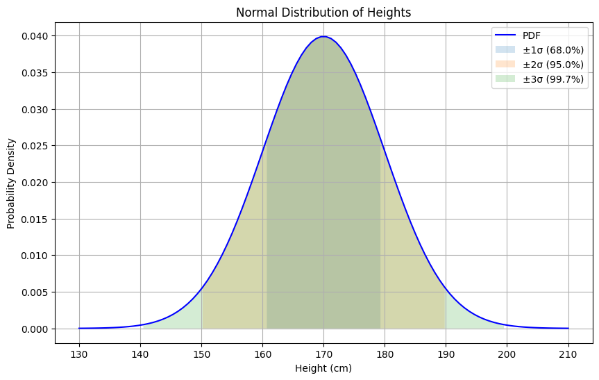
Common Applications
Section titled “Common Applications”-
Physical Measurements
- Height, weight
- Manufacturing dimensions
- Measurement errors
-
Natural Phenomena
- IQ scores
- Blood pressure
- Test scores
-
Financial Markets
- Stock returns
- Price fluctuations
- Risk modeling
Real-World Example: Quality Control
Section titled “Real-World Example: Quality Control”class ProductionLine: def __init__(self, target_length=100, tolerance=0.5): self.normal = NormalDistribution(target_length, tolerance/3) self.tolerance = tolerance
def produce_item(self): length = self.normal.simulate(1)[0] return { 'length': length, 'in_spec': abs(length - self.normal.mu) <= self.tolerance }
def analyze_batch(self, size=1000): batch = [self.produce_item() for _ in range(size)] defect_rate = 1 - sum(item['in_spec'] for item in batch) / size return f"Defect rate: {defect_rate:.2%}"
# Simulate productionline = ProductionLine()print(line.analyze_batch()) # Expected ≈ 0.20% defect rateZ-Score (Standard Score)
Section titled “Z-Score (Standard Score)”Z-score measures how many standard deviations away from the mean a data point is:
- Formula: z = (x - μ) / σ
- Standardizes any normal distribution to N(0,1)
- Useful for comparing values from different distributions
def calculate_z_score(x, mu, sigma):    return (x - mu) / sigma
# Exampleheight = 185  # cmz = calculate_z_score(height, mu=170, sigma=10)print(f"Z-score for {height}cm: {z:.2f}")  # 1.50print(f"Percentile: {norm.cdf(z):.2%}")    # 93.32%
Central Limit Theorem (CLT)
Section titled “Central Limit Theorem (CLT)”The CLT states that the sampling distribution of the mean approaches a normal distribution as sample size increases, regardless of the underlying distribution:
def demonstrate_clt(distribution, sample_size, n_samples):    means = [np.mean(distribution(sample_size))             for _ in range(n_samples)]    return means
# Example with uniform distributionuniform_samples = lambda n: np.random.uniform(0, 1, n)sample_means = demonstrate_clt(uniform_samples, 30, 1000)
plt.figure(figsize=(10, 6))plt.hist(sample_means, bins=30, density=True)plt.title('Sampling Distribution of Mean (n=30)')plt.xlabel('Sample Mean')plt.ylabel('Density')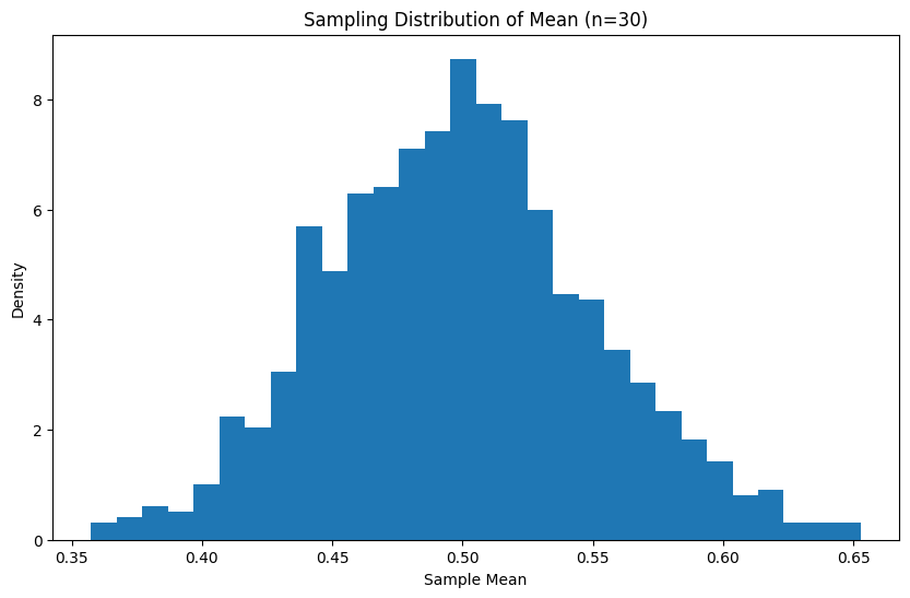
Key Points
Section titled “Key Points”-
Symmetry
- Perfectly symmetric around mean
- Skewness = 0
- Kurtosis = 3
-
Standardization
- Any normal distribution can be standardized
- Z-scores allow comparison across distributions
-
Empirical Rule
- 68-95-99.7 rule for data distribution
- Useful for quick probability estimates
-
Properties
- Sum of normal variables is normal
- Linear combination of normal variables is normal
- Independent of sample size (unlike t-distribution)
Standard Normal Distribution
Section titled “Standard Normal Distribution”The Standard Normal Distribution is a special case of the normal distribution where μ = 0 and σ = 1. It’s often denoted as N(0,1) and serves as a reference distribution.
Properties
Section titled “Properties”- Mean (μ) = 0
- Standard Deviation (σ) = 1
- PDF: f(z) = (1/√(2π)) * e^(-z²/2)
- Symmetric around zero
- Total area = 1
Z-Table Areas
Section titled “Z-Table Areas”- z = ±1: 68% of data
- z = ±2: 95% of data
- z = ±3: 99.7% of data
import numpy as npimport matplotlib.pyplot as pltfrom scipy.stats import norm
def plot_standard_normal():    z = np.linspace(-4, 4, 100)    pdf = norm.pdf(z, 0, 1)
    plt.figure(figsize=(10, 6))    plt.plot(z, pdf, 'b-', label='PDF')
    # Shade regions    colors = ['red', 'blue', 'green']    alphas = [0.1, 0.1, 0.1]    for i, (c, a) in enumerate(zip(colors, alphas), 1):        mask = (z >= -i) & (z <= i)        plt.fill_between(z[mask], pdf[mask], color=c, alpha=a,                        label=f'±{i}σ ({norm.cdf(i)-norm.cdf(-i):.1%})')
    plt.title('Standard Normal Distribution')    plt.xlabel('Z-Score')    plt.ylabel('Probability Density')    plt.grid(True)    plt.legend()    return plt
# Example usageplot = plot_standard_normal()plt.show()
Common Z-Score Values
Section titled “Common Z-Score Values”# Key probability pointsz_scores = { 0.90: 1.28, # 90% confidence 0.95: 1.96, # 95% confidence 0.99: 2.58 # 99% confidence}
# Example: Finding probabilitiesdef get_z_probability(z): return norm.cdf(z) - norm.cdf(-z)
print(f"P(-1 < Z < 1): {get_z_probability(1):.4f}") # 0.6827print(f"P(-2 < Z < 2): {get_z_probability(2):.4f}") # 0.9545print(f"P(-3 < Z < 3): {get_z_probability(3):.4f}") # 0.9973Applications
Section titled “Applications”- Standardization
def standardize(x, mu, sigma):return (x - mu) / sigma
Example: Test scores
Section titled “Example: Test scores”scores = [75, 82, 90, 68, 95] mu = np.mean(scores) sigma = np.std(scores) z_scores = [standardize(x, mu, sigma) for x in scores]
2. **Hypothesis Testing** ```python def z_test(sample_mean, pop_mean, pop_std, n): z = (sample_mean - pop_mean) / (pop_std / np.sqrt(n)) p_value = 2 * (1 - norm.cdf(abs(z))) # Two-tailed return z, p_value- Confidence Intervals
def confidence_interval(mean, std, n, confidence=0.95):z = norm.ppf((1 + confidence) / 2)margin = z * (std / np.sqrt(n))return mean - margin, mean + margin
Key Uses
Section titled “Key Uses”- Reference for normalizing data
- Base for statistical inference
- Quality control limits
- Risk assessment
- Hypothesis testing
Transformation
Section titled “Transformation”To convert between normal distributions:
- From N(μ,σ) to N(0,1): Z = (X - μ) / σ
- From N(0,1) to N(μ,σ): X = Zσ + μ
# Example: Converting between distributionsdef transform_distribution(x, from_params, to_params):    """    Transform value between normal distributions    from_params: tuple of (mean, std) of original distribution    to_params: tuple of (mean, std) of target distribution    """    from_mean, from_std = from_params    to_mean, to_std = to_params
    # First standardize    z = (x - from_mean) / from_std    # Then transform to new distribution    return z * to_std + to_mean
# Example usagex = 85  # Score from N(75, 10)new_x = transform_distribution(x, (75, 10), (100, 15))print(f"Score of {x} transforms to {new_x:.1f}")// Score of 85 transforms to 115.0
Uniform Distribution
Section titled “Uniform Distribution”The Uniform Distribution is a probability distribution where all outcomes in a given interval are equally likely to occur. It comes in two forms: discrete and continuous.
Types of Uniform Distributions
Section titled “Types of Uniform Distributions”-
Continuous Uniform Distribution
- Defined over continuous interval [a,b]
- Also called “rectangular distribution”
- Every point in interval has equal probability density
-
Discrete Uniform Distribution
- Defined over finite set of equally spaced values
- Each value has equal probability
- Example: Fair die (values 1-6)
Mathematical Properties
Section titled “Mathematical Properties”-
Continuous Uniform
- PDF: f(x) = 1/(b-a) for a ≤ x ≤ b, 0 otherwise
- CDF: F(x) = (x-a)/(b-a) for a ≤ x ≤ b
- Mean: μ = (a + b)/2
- Variance: σ² = (b - a)²/12
- Median: (a + b)/2
- Mode: Any value in [a,b]
- Skewness: 0 (symmetric)
- Kurtosis: 9/5 (platykurtic)
-
Discrete Uniform
- PMF:
P(X = x) = 1/n for each x in {x₁, ..., xₙ} - Mean:
(x₁ + xₙ)/2 - Variance:
(n² - 1)/12wherenis number of values
- PMF:
import numpy as npimport matplotlib.pyplot as pltfrom scipy.stats import uniform
class UniformDistribution:    def __init__(self, a=0, b=1):        self.a = a        self.b = b        self.mean = (a + b) / 2        self.variance = (b - a)**2 / 12        self.std = np.sqrt(self.variance)
    def pdf(self, x):        """Probability Density Function"""        return np.where((x >= self.a) & (x <= self.b),                       1/(self.b - self.a), 0)
    def cdf(self, x):        """Cumulative Distribution Function"""        return np.clip((x - self.a)/(self.b - self.a), 0, 1)
    def simulate(self, n_samples):        """Generate random samples"""        return np.random.uniform(self.a, self.b, n_samples)
# Visualization of PDF and CDFdef plot_uniform_distribution(a=0, b=1):    dist = UniformDistribution(a, b)    x = np.linspace(a-0.5, b+0.5, 1000)
    fig, (ax1, ax2) = plt.subplots(1, 2, figsize=(12, 4))
    # PDF    ax1.plot(x, dist.pdf(x))    ax1.fill_between(x, dist.pdf(x), alpha=0.3)    ax1.set_title('Probability Density Function')    ax1.grid(True)
    # CDF    ax2.plot(x, dist.cdf(x))    ax2.set_title('Cumulative Distribution Function')    ax2.grid(True)
    plt.tight_layout()    plt.show()
plot_uniform_distribution(0, 1)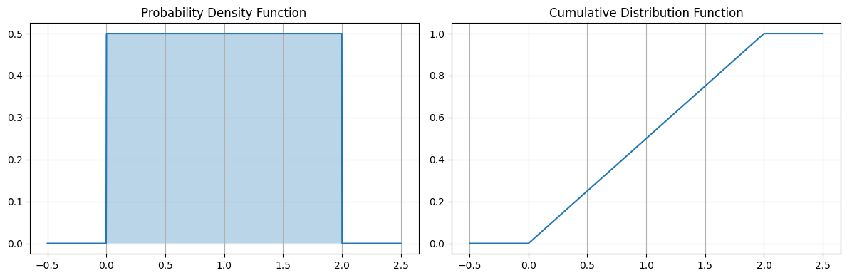
Applications and Examples
Section titled “Applications and Examples”- Random Number Generation
def random_number_generator(a, b, n=1):    """Generate n random numbers between a and b"""    uniform = UniformDistribution(a, b)    return uniform.simulate(n)
# Generate 5 random numbers between 0 and 10numbers = random_number_generator(0, 10, 5)print(f"Random numbers: {numbers}")- Simulation of Wait Times
class ServiceSimulator:    def __init__(self, min_time=5, max_time=15):        self.uniform = UniformDistribution(min_time, max_time)
    def simulate_service_times(self, n_customers):        times = self.uniform.simulate(n_customers)        return {            'times': times,            'average_wait': np.mean(times),            'total_time': np.sum(times)        }
# Simulate service times for 10 customerssimulator = ServiceSimulator()results = simulator.simulate_service_times(10)print(f"Average wait time: {results['average_wait']:.2f} minutes")// Average wait time: 10.21 minutes- Quality Control Bounds
class QualityControl:    def __init__(self, target, tolerance):        self.lower = target - tolerance        self.upper = target + tolerance        self.uniform = UniformDistribution(self.lower, self.upper)
    def check_production(self, n_items):        measurements = self.uniform.simulate(n_items)        in_spec = np.logical_and(            measurements >= self.lower,            measurements <= self.upper        )        return {            'measurements': measurements,            'pass_rate': np.mean(in_spec),            'failures': np.sum(~in_spec)
# Check 100 items with target 10 and tolerance ±0.5qc = QualityControl(target=10, tolerance=0.5)inspection = qc.check_production(100)print(f"Pass rate: {inspection['pass_rate']:.1%}")// Pass rate: 100.0%
Statistical Properties and Relationships
Section titled “Statistical Properties and Relationships”-
Sum of Uniform Variables
- Sum tends toward normal distribution (CLT)
- Special case: Irwin-Hall distribution
-
Order Statistics
- Minimum: a + (b-a)U₁/₍ₙ₊₁₎
- Maximum: a + (b-a)Uₙ/₍ₙ₊₁₎
- Where U follows Beta distribution
def demonstrate_sum_convergence(n_vars=12, n_samples=1000):    """Demonstrate convergence to normal as we sum uniforms"""    sums = np.sum([np.random.uniform(0, 1, n_samples)                   for _ in range(n_vars)], axis=0)
    plt.figure(figsize=(8, 4))    plt.hist(sums, bins=30, density=True)    plt.title(f'Sum of {n_vars} Uniform Variables')    plt.xlabel('Sum')    plt.ylabel('Density')    return plt
demonstrate_sum_convergence()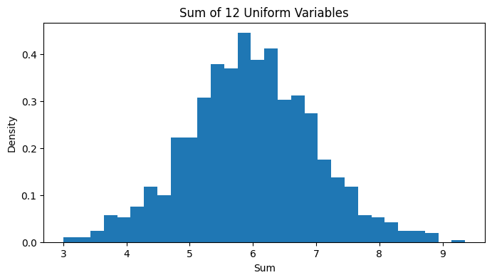
Hypothesis Testing with Uniform Distribution
Section titled “Hypothesis Testing with Uniform Distribution”The uniform distribution is often used in:
- Testing random number generators
- Goodness-of-fit tests
- P-value calculations
def test_uniformity(data, alpha=0.05):    """    Kolmogorov-Smirnov test for uniformity    """    from scipy import stats
    ks_stat, p_value = stats.kstest(data, 'uniform')    return {        'statistic': ks_stat,        'p_value': p_value,        'uniform': p_value > alpha    }
# Test random numbers for uniformitydata = np.random.uniform(0, 1, 1000)results = test_uniformity(data)print(f"Uniformity test p-value: {results['p_value']:.3f}")// Uniformity test p-value: 0.999
Key Points and Best Practices
Section titled “Key Points and Best Practices”-
When to Use
- Random sampling
- Simple probability models
- Null hypothesis testing
- Initial approximations
-
Limitations
- Assumes equal probability
- May oversimplify real phenomena
- Sensitive to interval bounds
-
Common Mistakes
- Assuming uniformity without testing
- Ignoring boundary effects
- Misinterpreting discrete vs continuous
Log Normal Distribution
Section titled “Log Normal Distribution”A Log Normal Distribution describes data where taking the natural log (ln) of the values gives a normal distribution. Think of it as a “skewed bell curve” that can’t go below zero.
Why It’s Important
Section titled “Why It’s Important”- Models things that grow by percentage (like money or populations)
- Always positive (can’t have negative values)
- Shows up naturally in many real-world situations
Key Features
Section titled “Key Features”- Skewed right (long tail on right side)
- Can’t be negative
- Most values cluster near the left
- Has a few very large values on the right
import numpy as npimport matplotlib.pyplot as pltfrom scipy.stats import lognorm
# Create simple example datanormal_data = np.random.normal(0, 0.5, 1000)lognormal_data = np.exp(normal_data)  # Transform to lognormal
# Plot both to show relationshipfig, (ax1, ax2) = plt.subplots(1, 2, figsize=(12, 5))
# Normal distribution plotax1.hist(normal_data, bins=30, density=True)ax1.set_title('Normal Distribution')ax1.set_xlabel('Value')
# Log normal distribution plotax2.hist(lognormal_data, bins=30, density=True)ax2.set_title('Log Normal Distribution')ax2.set_xlabel('Value')
plt.tight_layout()plt.show()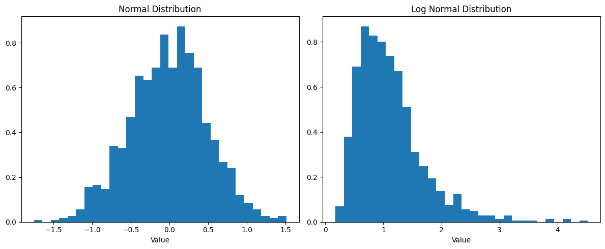
Real-World Examples
Section titled “Real-World Examples”- House Prices
def simulate_house_prices(median_price=300000, spread=0.5, n_houses=1000):    """Simulate house prices in a city"""    mu = np.log(median_price)  # Convert median to log scale    prices = np.random.lognormal(mu, spread, n_houses)
    return {        'median': np.median(prices),        'mean': np.mean(prices),        'cheapest': np.min(prices),        'most_expensive': np.max(prices)    }
# Exampleprices = simulate_house_prices()print(f"Median house: ${prices['median']:,.0f}")print(f"Average house: ${prices['mean']:,.0f}")print(f"Price range: ${prices['cheapest']:,.0f} to ${prices['most_expensive']:,.0f}")// Median house: $293,919// Average house: $334,266// Price range: $54,054 to $1,700,471- Investment Growth
def investment_scenarios(initial=10000, years=30, risk=0.15):    """Simulate possible investment outcomes"""    annual_return = 0.07  # 7% average return
    # Generate 1000 possible scenarios    final_amounts = initial * np.random.lognormal(        (annual_return - risk**2/2) * years,        risk * np.sqrt(years),        1000    )
    return {        'median': np.median(final_amounts),        'worst_10': np.percentile(final_amounts, 10),        'best_10': np.percentile(final_amounts, 90)    }
# Exampleresults = investment_scenarios()print(f"Typical outcome: ${results['median']:,.0f}")print(f"Range: ${results['worst_10']:,.0f} to ${results['best_10']:,.0f}")// Typical outcome: $60,900// Range: $19,375 to $173,670
When to Use It
Section titled “When to Use It”Use log normal when your data:
- Can’t be negative (like prices or sizes)
- Is skewed right (has a long tail to the right)
- Grows by percentages rather than fixed amounts
Simple Rules of Thumb
Section titled “Simple Rules of Thumb”- Most values will be below the mean
- Median is less than mean
- A few very large values will pull the mean up
- Multiplying/dividing by a constant shifts the distribution
Common Mistakes to Avoid
Section titled “Common Mistakes to Avoid”- Using it for negative values (impossible)
- Expecting symmetry (it’s always skewed)
- Using regular averages (use geometric mean instead)
- Forgetting to transform back from log scale
# Example showing common statisticsdef log_normal_stats(data):    """Calculate key statistics for log-normal data"""    log_data = np.log(data)
    return {        'median': np.exp(np.mean(log_data)),  # Geometric mean        'mean': np.mean(data),                # Arithmetic mean        'typical_range': [            np.exp(np.mean(log_data) - np.std(log_data)),            np.exp(np.mean(log_data) + np.std(log_data))        ]    }
# Example with salary datasalaries = np.random.lognormal(11, 0.5, 1000)  # Generate sample salariesstats = log_normal_stats(salaries)
print(f"Typical salary (median): ${stats['median']:,.0f}")print(f"Average salary (mean): ${stats['mean']:,.0f}")print(f"Typical range: ${stats['typical_range'][0]:,.0f} to ${stats['typical_range'][1]:,.0f}")// Typical salary (median): $31,623// Average salary (mean): $34,859// Typical range: $25,262 to $41,771Remember: Log normal distributions are perfect for things that grow by percentages (like money) or can’t be negative (like sizes or times).
Power Law Distribution/Pareto Distribution
Section titled “Power Law Distribution/Pareto Distribution”The Power Law Distribution (also known as Pareto Distribution) describes situations where a small number of items dominate the majority of outcomes. It’s often called the “80/20 rule” - where 80% of effects come from 20% of causes.
Key Properties
Section titled “Key Properties”- Long tail distribution (many small values, few very large ones)
- No typical scale (looks similar at different scales)
- Formula: P(x) ∝ x^(-α) where α > 0
- Common α values: 2-3 for natural phenomena
Real-World Examples
Section titled “Real-World Examples”- Wealth distribution (few people own most wealth)
- City populations (few cities have most people)
- Website traffic (few pages get most visits)
- Social media followers (few accounts have most followers)
import numpy as npimport matplotlib.pyplot as plt
def plot_power_law(alpha=2, n_samples=1000):    # Generate power law data    x = np.random.pareto(alpha, n_samples) + 1
    # Plot on log-log scale    plt.figure(figsize=(10, 6))    plt.hist(x, bins=50, density=True, alpha=0.7)    plt.yscale('log')    plt.xscale('log')    plt.title(f'Power Law Distribution (α={alpha})')    plt.xlabel('Value (log scale)')    plt.ylabel('Frequency (log scale)')    plt.grid(True)    return plt
# Example usageplot_power_law()plt.show()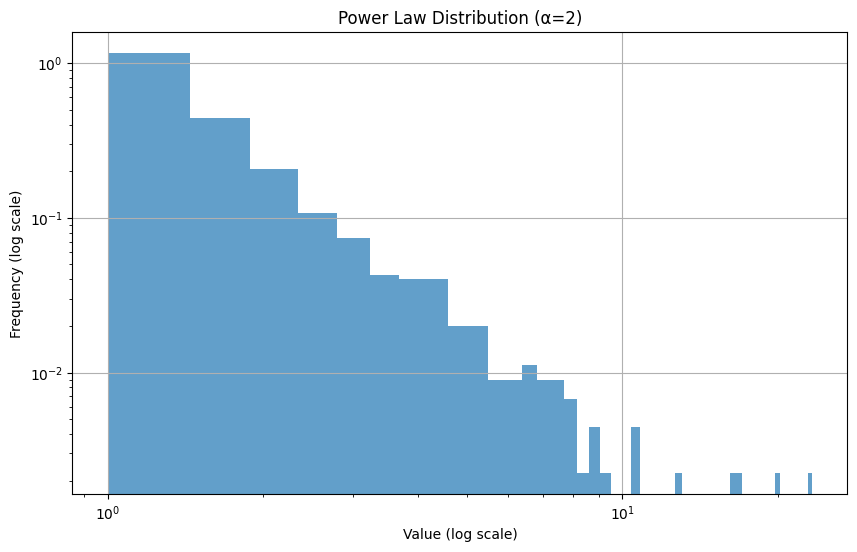
Simple Example: Website Traffic
Section titled “Simple Example: Website Traffic”def simulate_website_traffic(n_pages=100): """Simulate daily views for website pages""" # Generate power law distributed views views = np.random.pareto(2, n_pages) * 100
# Sort and analyze sorted_views = np.sort(views)[::-1] # Descending order total_views = np.sum(views)
# Find 80/20 point cumsum = np.cumsum(sorted_views) pages_for_80 = np.searchsorted(cumsum, 0.8 * total_views) + 1
return { 'top_pages': sorted_views[:5], 'pages_for_80_percent': pages_for_80, 'percent_pages': (pages_for_80 / n_pages) * 100 }
# Exampletraffic = simulate_website_traffic()print(f"Top 5 page views: {traffic['top_pages'].astype(int)}")print(f"{traffic['pages_for_80_percent']} pages ({traffic['percent_pages']:.1f}%) " f"generate 80% of traffic")// Top 5 page views: [449 396 388 277 272]// 40 pages (40.0%) generate 80% of trafficWhen to Use
Section titled “When to Use”- Analyzing extreme inequalities
- Modeling natural phenomena
- Risk assessment
- Network analysis
Key Points
Section titled “Key Points”- No “typical” or “average” value
- Extreme values are more common than in normal distribution
- Often indicates self-reinforcing processes
- Important for risk management (extreme events more likely)
Note: Power laws appear in many natural and social systems. If you see huge differences between largest and smallest values, consider using a power law distribution.
Inferential Statistics
Section titled “Inferential Statistics”Estimates
Section titled “Estimates”Estimates are predictions or approximations of unknown values in data science. They help us make informed decisions based on available data.
Types of Estimates
Section titled “Types of Estimates”-
Point Estimate
- Single value prediction
- Example: Sample mean (x̄) estimates population mean (μ)
data = [1, 2, 3, 4, 5]point_estimate = np.mean(data) # = 3 -
Interval Estimate
- Range of likely values
- Common form: Confidence Intervals
def confidence_interval(data, confidence=0.95):mean = np.mean(data)std = np.std(data, ddof=1)margin = 1.96 * (std / np.sqrt(len(data))) # 95% CIreturn mean - margin, mean + margin
Common Estimators
Section titled “Common Estimators”-
Mean (Average)
- Estimates central tendency
- Best for symmetric data
mean = sum(data) / len(data) -
Median
- Estimates central value
- Better for skewed data
median = sorted(data)[len(data)//2] -
Sample Variance
- Estimates data spread
- Uses n-1 for unbiased estimate
variance = sum((x - mean)**2 for x in data) / (len(data) - 1)
Properties of Good Estimators
Section titled “Properties of Good Estimators”-
Unbiased
- Average estimate equals true value
- Example: Sample mean is unbiased
-
Consistent
- More data = better estimate
- Example: Law of large numbers
-
Efficient
- Minimum variance among similar estimators
- Example: Sample mean vs single observation
Real-World Example
Section titled “Real-World Example”class SalesEstimator: def __init__(self, sales_data): self.data = sales_data
def daily_estimate(self): mean = np.mean(self.data) ci = confidence_interval(self.data) return { 'point_estimate': mean, 'confidence_interval': ci, 'reliability': 'High' if (ci[1]-ci[0]) < mean*0.2 else 'Low' }
# Usagesales = [100, 120, 80, 95, 110, 105, 90]estimator = SalesEstimator(sales)forecast = estimator.daily_estimate()print(f"Expected sales: {forecast['point_estimate']:.0f}")print(f"Range: {forecast['confidence_interval'][0]:.0f} to {forecast['confidence_interval'][1]:.0f}")// Expected sales: 100// Range: 90 to 110Key Point: Choose estimators based on your data type and what you’re trying to predict.
Hypothesis Testing
Section titled “Hypothesis Testing”Hypothesis testing is a method to make decisions about a population using sample data. It helps determine if an observed effect is statistically significant.
Basic Steps
Section titled “Basic Steps”-
State Hypotheses
- Null (H₀): No effect/relationship exists
- Alternative (H₁): Effect/relationship exists
-
Choose Significance Level (α)
- Usually 0.05 (5%)
- Represents acceptable false positive rate
-
Calculate Test Statistic
- Based on sample data
- Common tests: z-test, t-test
-
Compare p-value
- If p < α: Reject H₀
- If p ≥ α: Fail to reject H₀
Simple Example
Section titled “Simple Example”from scipy import stats
# Test if mean score is different from 70scores = [72, 75, 68, 77, 69, 71, 74, 73]
# Run t-testt_stat, p_value = stats.ttest_1samp(scores, 70)
print(f"p-value: {p_value:.4f}")if p_value < 0.05: print("Reject null hypothesis")else: print("Fail to reject null hypothesis")
// p-value: 0.0615// Fail to reject null hypothesisCommon Tests
Section titled “Common Tests”-
One-Sample t-test
- Compare sample mean to known value
def one_sample_ttest(data, expected_mean, alpha=0.05):t_stat, p_val = stats.ttest_1samp(data, expected_mean)return {'p_value': p_val,'significant': p_val < alpha,'test_stat': t_stat} -
Two-Sample t-test
- Compare means of two groups
def two_sample_ttest(group1, group2, alpha=0.05):t_stat, p_val = stats.ttest_ind(group1, group2)return {'p_value': p_val,'significant': p_val < alpha,'test_stat': t_stat} -
Chi-Square Test
- Test categorical data relationships
def chi_square_test(observed, expected, alpha=0.05):chi2, p_val = stats.chisquare(observed, expected)return {'p_value': p_val,'significant': p_val < alpha,'test_stat': chi2}
Real-World Example
Section titled “Real-World Example”class DrugEffectTest: def __init__(self, treatment_group, control_group): self.treatment = treatment_group self.control = control_group
def analyze(self): # Run t-test result = two_sample_ttest(self.treatment, self.control)
# Calculate effect size effect = np.mean(self.treatment) - np.mean(self.control)
return { 'significant': result['significant'], 'p_value': result['p_value'], 'effect_size': effect, 'recommendation': 'Use drug' if (result['significant'] and effect > 0) else 'Need more research' }
# Example usagetreatment = [75, 82, 78, 80, 79] # Drug groupcontrol = [70, 71, 73, 69, 72] # Placebo group
test = DrugEffectTest(treatment, control)result = test.analyze()
print(f"Effect: {result['effect_size']:.1f} units")print(f"P-value: {result['p_value']:.4f}")print(f"Recommendation: {result['recommendation']}")// Effect: 7.8 units// P-value: 0.0004// Recommendation: Use drugCommon Mistakes to Avoid
Section titled “Common Mistakes to Avoid”-
P-value Misinterpretation
- P-value is NOT probability H₀ is true
- Only shows how rare data is under H₀
-
Multiple Testing
- More tests = higher chance of false positives
- Use Bonferroni correction: α/n for n tests
-
Sample Size Issues
- Too small: May miss real effects
- Too large: May find tiny, meaningless effects
Key Point: Hypothesis testing helps make decisions but should be used with context and common sense.
P Value
Section titled “P Value”P-value helps determine if a result is statistically significant. Think of it as “how surprising is this result if there was no real effect?”
Key Points
Section titled “Key Points”- Smaller p-value = stronger evidence against null hypothesis
- Common threshold: p < 0.05 (5% significance level)
- Range: 0 to 1 (0% to 100% probability)
Simple Example
Section titled “Simple Example”from scipy import statsimport numpy as np
# Test if coin is fairflips = [1, 1, 1, 1, 1, 1, 1, 0, 0, 0] # 1=heads, 0=tailsheads = sum(flips)total = len(flips)
# Calculate p-value (two-tailed test)result = stats.binomtest(heads, total, p=0.5)p_value = result.pvalue
# Print resultsprint(f"Number of heads: {heads} out of {total}")print(f"P-value: {p_value:.3f}")print(f"Interpretation: {'Reject null hypothesis' if p_value < 0.05 else 'Fail to reject null hypothesis'}")
# In this case:# H0: Coin is fair (p = 0.5)# H1: Coin is biased (p ≠ 0.5)# Since p-value (0.344) > 0.05, we fail to reject H0
// Number of heads: 7 out of 10// P-value: 0.344// Interpretation: Fail to reject null hypothesisInterpretation Guide
Section titled “Interpretation Guide”- p < 0.01: Very strong evidence
- p < 0.05: Strong evidence
- p < 0.10: Weak evidence
- p ≥ 0.10: No evidence
Common Mistakes
Section titled “Common Mistakes”-
P-value is NOT:
- Probability null hypothesis is true
- Probability of being wrong
- Effect size or importance
-
Small p-value doesn’t mean:
- Large effect
- Practical significance
- Reproducible results
Remember: P-value measures evidence strength, not effect size or practical importance
Z Test
Section titled “Z Test”A Z-test is a statistical test used to determine if there’s a significant difference between a sample mean and a population mean when:
- Population standard deviation is known
- Sample size is large (n > 30)
Formula
Section titled “Formula”z = (x̄ - μ) / (σ / √n)
where:x̄ = sample meanμ = population meanσ = population standard deviationn = sample sizeSimple Example
Section titled “Simple Example”import numpy as npfrom scipy import stats
def z_test(sample, pop_mean, pop_std): """ Perform one-sample z-test
Args: sample: List of sample values pop_mean: Known population mean pop_std: Known population standard deviation """ n = len(sample) sample_mean = np.mean(sample) z_score = (sample_mean - pop_mean) / (pop_std / np.sqrt(n)) p_value = 2 * (1 - stats.norm.cdf(abs(z_score))) # Two-tailed test
return { 'z_score': z_score, 'p_value': p_value, 'significant': p_value < 0.05 }
# Example: Test if class scores are different from populationscores = [85, 88, 92, 78, 90, 87, 86, 84, 89, 91] # Sample scorespop_mean = 82 # Known population meanpop_std = 5 # Known population standard deviation
result = z_test(scores, pop_mean, pop_std)print(f"Z-score: {result['z_score']:.2f}")print(f"P-value: {result['p_value']:.4f}")print(f"Significant? {result['significant']}")
// Z-score: 3.16// P-value: 0.0016// Significant? TrueWhen to Use Z-Test
Section titled “When to Use Z-Test”- Large sample size (n > 30)
- Known population standard deviation
- Testing means (not proportions)
- Data is normally distributed
Real-World Example: Quality Control
Section titled “Real-World Example: Quality Control”class ProductQuality: def __init__(self, target_weight=100, pop_std=2): self.target = target_weight self.pop_std = pop_std
def test_batch(self, measurements): result = z_test(measurements, self.target, self.pop_std) return { 'pass': not result['significant'], # Pass if no significant difference 'z_score': result['z_score'], 'p_value': result['p_value'] }
# Test a batch of productsweights = [101, 99, 100, 102, 98, 101, 99, 100, 101, 102]qc = ProductQuality()test = qc.test_batch(weights)
print(f"Batch {'passed' if test['pass'] else 'failed'} quality check")print(f"Z-score: {test['z_score']:.2f}")
// Batch passed quality check// Z-score: 0.47Key Points
Section titled “Key Points”-
Assumptions
- Normal distribution
- Independent samples
- Known population standard deviation
-
Interpretation
- |Z| > 1.96: Significant at 5% level
- |Z| > 2.58: Significant at 1% level
- Larger |Z| = stronger evidence
-
Limitations
- Requires known population std
- Not good for small samples
- Assumes normality
Note: If population standard deviation is unknown or sample size is small, use t-test instead.
Student’s t Distribution
Section titled “Student’s t Distribution”The Student’s t Distribution is similar to the normal distribution but has heavier tails. It’s used when:
- Sample size is small (n < 30)
- Population standard deviation is unknown
Key Points
Section titled “Key Points”- Shape depends on degrees of freedom (df = n-1)
- Approaches normal distribution as df increases
- Used for t-tests and confidence intervals
Formula
Section titled “Formula”from scipy import statsimport numpy as np
def t_distribution(df, x): """Calculate t-distribution probability density""" return stats.t.pdf(x, df)Example: Compare t vs Normal
Section titled “Example: Compare t vs Normal”import matplotlib.pyplot as plt
# Create comparison plotx = np.linspace(-4, 4, 100)df_values = [1, 5, 30]
plt.figure(figsize=(10, 6))for df in df_values: plt.plot(x, stats.t.pdf(x, df), label=f't (df={df})')
plt.plot(x, stats.norm.pdf(x), label='Normal', linestyle='--')plt.title('t Distribution vs Normal')plt.legend()plt.grid(True)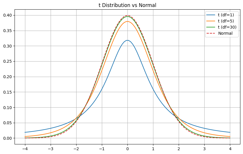
Common Uses
Section titled “Common Uses”- Small Sample Testing
def t_test(sample, pop_mean):    """One-sample t-test"""    t_stat, p_value = stats.ttest_1samp(sample, pop_mean)    return {        't_statistic': t_stat,        'p_value': p_value,        'significant': p_value < 0.05    }
# Exampledata = [25, 28, 29, 30, 31]result = t_test(data, 27)print(f"P-value: {result['p_value']:.4f}")
// P-value: 0.1951- Confidence Intervals
def confidence_interval(data, confidence=0.95):    """Calculate confidence interval"""    n = len(data)    mean = np.mean(data)    sem = stats.sem(data)  # Standard error of mean    interval = stats.t.interval(confidence, n-1, mean, sem)    return interval
# Exampledata = [10, 12, 11, 13, 9]ci = confidence_interval(data)print(f"95% CI: ({ci[0]:.1f}, {ci[1]:.1f})")
// 95% CI: (9.0, 13.0)
When to Use
Section titled “When to Use”- Small sample sizes
- Unknown population standard deviation
- Testing means or differences
- Creating confidence intervals
Key Differences from Normal Distribution
Section titled “Key Differences from Normal Distribution”- More spread out (heavier tails)
- Changes shape with sample size
- More conservative (wider intervals)
- Better for small samples
Note: As sample size increases (n > 30), t-distribution becomes very close to normal distribution.
T-Stats with T-test Hypothesis Testing
Section titled “T-Stats with T-test Hypothesis Testing”T-tests help determine if there’s a significant difference between means. They’re especially useful when working with small samples (n < 30).
Basic Types of T-tests
Section titled “Basic Types of T-tests”-
One-Sample T-test
- Compares sample mean to known value
from scipy import stats# Example: Test if student scores differ from target (75)scores = [72, 78, 75, 80, 73]t_stat, p_value = stats.ttest_1samp(scores, 75) -
Independent T-test
- Compares means of two independent groups
# Compare treatment vs controltreatment = [75, 82, 78, 80]control = [70, 71, 73, 69]t_stat, p_value = stats.ttest_ind(treatment, control) -
Paired T-test
- Compares before/after measurements
# Compare before/after scoresbefore = [70, 72, 71, 73]after = [75, 78, 77, 76]t_stat, p_value = stats.ttest_rel(before, after)
Simple Example with Explanation
Section titled “Simple Example with Explanation”def run_ttest(sample_data, expected_mean=0, alpha=0.05): """ Run one-sample t-test
Args: sample_data: List of values expected_mean: Value to test against alpha: Significance level """ # Calculate t-statistic and p-value t_stat, p_value = stats.ttest_1samp(sample_data, expected_mean)
return { 't_statistic': t_stat, 'p_value': p_value, 'significant': p_value < alpha, 'mean_difference': np.mean(sample_data) - expected_mean }
# Example usagescores = [85, 82, 88, 84, 86]result = run_ttest(scores, expected_mean=80)
print(f"T-statistic: {result['t_statistic']:.2f}")print(f"P-value: {result['p_value']:.4f}")print(f"Mean difference: {result['mean_difference']:.1f}")print(f"Significant? {result['significant']}")
// T-statistic: 5.00// P-value: 0.0075// Mean difference: 5.0// Significant? TrueWhen to Use Each Test
Section titled “When to Use Each Test”-
One-Sample T-test
- Testing against known value
- Example: Are test scores different from 70?
-
Independent T-test
- Comparing two separate groups
- Example: Does treatment group differ from control?
-
Paired T-test
- Before/after measurements
- Example: Did training improve scores?
Interpreting Results
Section titled “Interpreting Results”-
T-statistic
- Larger = stronger evidence
- Sign shows direction (positive/negative)
-
P-value
- < 0.05: Statistically significant
- ≥ 0.05: Not significant
-
Effect Size
- Mean difference shows practical significance
- Consider alongside p-value
Common Mistakes to Avoid
Section titled “Common Mistakes to Avoid”-
Don’t ignore assumptions:
- Normal distribution
- Independent samples
- Equal variances (for independent t-test)
-
Don’t rely only on p-values:
def analyze_results(result):"""Better interpretation of t-test"""return {'statistical_sig': result['p_value'] < 0.05,'practical_sig': abs(result['mean_difference']) > 5,'recommendation': 'Consider both statistical and practical significance'}
Real-World Example
Section titled “Real-World Example”class DrugEffectiveness: def __init__(self, treatment_data, control_data): self.treatment = treatment_data self.control = control_data
def analyze(self): # Run t-test t_stat, p_val = stats.ttest_ind(self.treatment, self.control)
# Calculate effect size effect = np.mean(self.treatment) - np.mean(self.control)
return { 't_statistic': t_stat, 'p_value': p_val, 'effect_size': effect, 'recommendation': 'Effective' if (p_val < 0.05 and effect > 0) else 'Not effective' }
# Example usagetreatment = [95, 92, 98, 94, 96] # Drug groupcontrol = [85, 87, 88, 86, 84] # Placebo group
study = DrugEffectiveness(treatment, control)results = study.analyze()
print(f"Effect size: {results['effect_size']:.1f} units")print(f"P-value: {results['p_value']:.4f}")print(f"Recommendation: {results['recommendation']}")
// Effect size: 9.0 units// P-value: 0.0001// Recommendation: EffectiveKey Points:
- Use t-tests for small samples
- Consider both p-value and effect size
- Check assumptions before testing
- Interpret results in context
T-test vs Z-test
Section titled “T-test vs Z-test”T-tests and Z-tests are both used to compare means, but they have different use cases and assumptions.
Quick Reference
Section titled “Quick Reference”| Feature | Z-test | T-test |
|---|---|---|
| Sample Size | Large (n > 30) | Any size |
| Population σ | Must be known | Can be unknown |
| Distribution | Normal | Student’s t |
| Tail Weight | Light tails | Heavy tails |
Simple Example
Section titled “Simple Example”import numpy as npfrom scipy import stats
def choose_test(sample, pop_mean, pop_std=None): """ Choose and run appropriate test
Args: sample: Data to test pop_mean: Population mean to test against pop_std: Population standard deviation (if known) """ n = len(sample)
if n > 30 and pop_std is not None: # Use Z-test z_score = (np.mean(sample) - pop_mean) / (pop_std / np.sqrt(n)) p_value = 2 * (1 - stats.norm.cdf(abs(z_score))) test_type = 'Z-test' stat = z_score else: # Use T-test stat, p_value = stats.ttest_1samp(sample, pop_mean) test_type = 'T-test'
return { 'test_type': test_type, 'statistic': stat, 'p_value': p_value }
# Example usagesmall_sample = [75, 82, 78, 80, 79] # n = 5large_sample = np.random.normal(75, 5, 50) # n = 50pop_std = 5
# Test both samplessmall_result = choose_test(small_sample, 70)large_result = choose_test(large_sample, 70, pop_std)
print(f"Small sample: {small_result['test_type']}")print(f"Large sample: {large_result['test_type']}")
// Small sample: T-test// Large sample: Z-testWhen to Use Each Test
Section titled “When to Use Each Test”-
Use Z-test when:
- Large sample (n > 30)
- Known population standard deviation
- Need exact probability values
-
Use T-test when:
- Small sample size
- Unknown population standard deviation
- Working with sample statistics
Key Differences
Section titled “Key Differences”-
Tail Weight
- Z-test: Lighter tails (normal distribution)
- T-test: Heavier tails (more conservative)
-
Critical Values
- Z-test: Fixed values (e.g., ±1.96 for 95%)
- T-test: Varies with sample size (degrees of freedom)
-
Confidence Intervals
def compare_intervals(data, pop_std=None, confidence=0.95):    """Compare Z and T confidence intervals"""    n = len(data)    mean = np.mean(data)
    # Z interval (if pop_std known)    if pop_std:        z = stats.norm.ppf((1 + confidence) / 2)        z_margin = z * (pop_std / np.sqrt(n))        z_interval = (mean - z_margin, mean + z_margin)
    # T interval    t_interval = stats.t.interval(confidence, n-1, mean, stats.sem(data))
    return {        'z_interval': z_interval if pop_std else None,        't_interval': t_interval    }
Best Practices
Section titled “Best Practices”-
Default to T-test unless you:
- Have large sample AND
- Know population standard deviation
-
Consider Sample Size
- Small (n < 30): Always use t-test
- Large (n > 30): Either test works
-
Check Assumptions
- Normal distribution
- Independent observations
- Random sampling
Note: When in doubt, use t-test. It’s more conservative and safer for most situations.
Type I and Type II Errors
Section titled “Type I and Type II Errors”Type I and Type II errors are fundamental concepts in hypothesis testing that help us understand the two ways we can make mistakes.
Quick Reference
Section titled “Quick Reference”| Error Type | Definition | Common Name | Example |
|---|---|---|---|
| Type I | Rejecting true null hypothesis | False Positive | Convicting innocent person |
| Type II | Failing to reject false null hypothesis | False Negative | Missing actual disease |
Simple Example
Section titled “Simple Example”import numpy as npfrom scipy import stats
def test_with_errors(data, null_mean, alpha=0.05): """ Run hypothesis test and explain possible errors
Args: data: Sample data null_mean: Null hypothesis mean alpha: Significance level (Type I error rate) """ # Run t-test t_stat, p_value = stats.ttest_1samp(data, null_mean)
# Decision reject_null = p_value < alpha
# Explain possible errors if reject_null: error_type = "Type I error possible (false positive)" else: error_type = "Type II error possible (false negative)"
return { 'p_value': p_value, 'reject_null': reject_null, 'possible_error': error_type }
# Examplescores = [75, 82, 78, 80, 79]result = test_with_errors(scores, null_mean=70)print(f"Decision: {'Reject' if result['reject_null'] else 'Fail to reject'} null")print(f"Possible error: {result['possible_error']}")
// Decision: Reject null// Possible error: Type I error possible (false positive)Key Concepts
Section titled “Key Concepts”-
Type I Error (α)
- Rejecting H₀ when it’s true
- Probability = significance level (α)
- Usually set to 0.05 (5%)
- More serious in legal/medical contexts
-
Type II Error (β)
- Not rejecting H₀ when it’s false
- Related to test power (1 - β)
- Affected by:
- Sample size
- Effect size
- Significance level
Real-World Example: Medical Test
Section titled “Real-World Example: Medical Test”class MedicalTest: def __init__(self, sensitivity=0.95, specificity=0.98): self.sensitivity = sensitivity # True Positive Rate self.specificity = specificity # True Negative Rate
def test_patient(self, has_disease, n_tests=1000): """Simulate medical tests""" if has_disease: # Type II error rate = 1 - sensitivity false_negatives = np.random.binomial(n_tests, 1-self.sensitivity) return { 'condition': 'Sick', 'errors': false_negatives, 'error_type': 'Type II', 'error_rate': false_negatives/n_tests } else: # Type I error rate = 1 - specificity false_positives = np.random.binomial(n_tests, 1-self.specificity) return { 'condition': 'Healthy', 'errors': false_positives, 'error_type': 'Type I', 'error_rate': false_positives/n_tests }
# Example usagetest = MedicalTest()sick_results = test.test_patient(has_disease=True)healthy_results = test.test_patient(has_disease=False)
print(f"Type II Error Rate (missed disease): {sick_results['error_rate']:.1%}")print(f"Type I Error Rate (false alarms): {healthy_results['error_rate']:.1%}")
// Type II Error Rate (missed disease): 5.7%// Type I Error Rate (false alarms): 2.2%Trade-offs
Section titled “Trade-offs”-
Error Rate Relationship
- Decreasing α increases β
- Decreasing β increases α
- Can’t minimize both simultaneously
-
Practical Considerations
- Cost of each error type
- Available sample size
- Required confidence level
Common Mistakes to Avoid
Section titled “Common Mistakes to Avoid”-
Not Considering Both Errors
def assess_test_quality(alpha, beta):"""Evaluate overall test quality"""power = 1 - betareturn {'false_positive_rate': alpha,'false_negative_rate': beta,'power': power,'quality': 'Good' if (alpha < 0.05 and power > 0.8) else 'Poor'} -
Focusing Only on Significance
- Consider practical significance
- Balance both error types
- Account for sample size
Key Point: Always consider both error types and their real-world implications when making decisions based on statistical tests.
Conclusion
Section titled “Conclusion”Understanding Type I and Type II errors is crucial for making informed decisions in data analysis. By balancing these errors, we can improve the reliability and practicality of our statistical tests.
Remember, the goal is not to minimize errors, but to make informed decisions with the best possible information.
Summary
Section titled “Summary”- Type I Error: Rejecting true null hypothesis
- Type II Error: Failing to reject false null hypothesis
- Trade-offs: Can’t minimize both simultaneously
- Practical Considerations: Cost, sample size, confidence level
- Common Mistakes: Focusing only on significance
Key Point: Always consider both error types and their real-world implications when making decisions based on statistical tests.
Bayesian Statistics
Section titled “Bayesian Statistics”Bayesian statistics is an approach that updates beliefs based on new evidence. It uses probability to express uncertainty about events and parameters.
Key Concepts
Section titled “Key Concepts”-
Prior Probability (Prior)
- Initial belief before new data
- Based on previous knowledge
-
Likelihood
- Probability of data given parameters
- How well parameters explain data
-
Posterior Probability
- Updated belief after seeing data
- Combines prior and likelihood
Bayes’ Theorem
Section titled “Bayes’ Theorem”The fundamental formula:
P(A|B) = P(B|A) * P(A) / P(B)
where:P(A|B) = PosteriorP(B|A) = LikelihoodP(A) = PriorP(B) = Evidence
Simple Example
Section titled “Simple Example”def bayes_update(prior_prob, likelihood, evidence): """Calculate posterior probability""" return (likelihood * prior_prob) / evidence
# Example: Disease testingprior = 0.01 # 1% have diseaselikelihood = 0.95 # Test 95% accurate for sick peopleevidence = 0.05 # 5% test positive
posterior = bayes_update(prior, likelihood, evidence)print(f"Probability of disease given positive test: {posterior:.1%}")// Probability of disease given positive test: 19.0%Real-World Applications
Section titled “Real-World Applications”- Spam Detection
class SpamFilter:    def __init__(self):        self.word_probs = {            'money': 0.8,    # P(spam|word)            'friend': 0.2,            'buy': 0.7        }        self.spam_prior = 0.3  # 30% of emails are spam
    def classify(self, words):        prob = self.spam_prior        for word in words:            if word in self.word_probs:                prob *= self.word_probs[word]        return prob > 0.5
# Examplefilter = SpamFilter()email = ['money', 'buy']is_spam = filter.classify(email)print(f"Email classified as: {'Spam' if is_spam else 'Not Spam'}")// Email classified as: Not Spam- A/B Testing
def bayesian_ab_test(a_success, a_total, b_success, b_total):    """Compare two versions using Bayesian approach"""    from scipy import stats
    # Calculate success rates    rate_a = a_success / a_total    rate_b = b_success / b_total
    # Calculate confidence    confidence = stats.beta(a_success + 1, a_total - a_success + 1).mean()
    return {        'better_version': 'A' if rate_a > rate_b else 'B',        'confidence': confidence,        'recommend_switch': confidence > 0.95    }
# Exampleresult = bayesian_ab_test(120, 1000, 150, 1000)print(f"Better version: {result['better_version']}")print(f"Confidence: {result['confidence']:.1%}")// Better version: B// Confidence: 98.2%
Advantages Over Frequentist Statistics
Section titled “Advantages Over Frequentist Statistics”-
Intuitive Updates
- Naturally updates beliefs with new data
- Handles uncertainty better
-
Prior Knowledge
- Incorporates existing knowledge
- More realistic in real-world scenarios
-
Interpretable Results
- Gives probability distributions
- Easier to understand for decisions
Common Uses
Section titled “Common Uses”-
Medical Diagnosis
- Update disease probability with test results
- Consider patient history (prior)
-
Machine Learning
- Parameter estimation
- Model uncertainty
- Neural network weights
-
Risk Assessment
- Financial decisions
- Project planning
- Insurance
Simple Implementation
Section titled “Simple Implementation”class BayesianAnalyzer: def __init__(self, prior=0.5): self.prior = prior self.data = []
def update(self, new_data, likelihood): """Update beliefs with new data""" posterior = (likelihood * self.prior) / ( likelihood * self.prior + (1 - likelihood) * (1 - self.prior) ) self.prior = posterior self.data.append(new_data) return posterior
def get_confidence(self): return f"{self.prior:.1%}"
# Example usageanalyzer = BayesianAnalyzer()print(f"Initial belief: {analyzer.get_confidence()}")
# Update with new evidenceevidence = [True, True, False, True]for e in evidence: likelihood = 0.8 if e else 0.2 analyzer.update(e, likelihood)
print(f"Updated belief: {analyzer.get_confidence()}")// Initial belief: 50.0%// Updated belief: 94.1%Key Points to Remember
Section titled “Key Points to Remember”-
Start with Prior
- Use existing knowledge
- Be explicit about assumptions
-
Update with Data
- Use Bayes’ theorem
- Consider evidence strength
-
Make Decisions
- Use posterior probabilities
- Consider uncertainty
Note: Bayesian statistics helps make better decisions by combining prior knowledge with new evidence in a natural way.
Conclusion
Section titled “Conclusion”Bayesian statistics is a powerful tool for making decisions based on uncertain data. It provides a natural way to update beliefs with new evidence and can be used in a wide range of applications.
By understanding the basics and practicing with real-world examples, you can start using Bayesian methods to improve your decision-making process.
Summary
Section titled “Summary”- Bayes’ Theorem: P(A|B) = P(B|A) * P(A) / P(B)
- Prior: Initial belief
- Likelihood: Data explanation
- Posterior: Updated belief
- Common Uses: Medical, ML, risk assessment
Key Point: Bayesian statistics helps make better decisions by combining prior knowledge with new evidence in a natural way.
Confidence Interval and Margin of Error
Section titled “Confidence Interval and Margin of Error”A confidence interval shows the likely range for a population value, while margin of error shows how far the estimate might be from the true value.
Simple Formula
Section titled “Simple Formula”margin_of_error = z_score * (standard_deviation / √sample_size)confidence_interval = sample_mean ± margin_of_errorBasic Example
Section titled “Basic Example”import numpy as npfrom scipy import stats
def calculate_confidence_interval(data, confidence=0.95): """ Calculate confidence interval for a dataset
Args: data: List of numbers confidence: Confidence level (default 95%) """ mean = np.mean(data) std_error = stats.sem(data) interval = stats.t.interval(confidence, len(data)-1, mean, std_error)
return { 'mean': mean, 'lower': interval[0], 'upper': interval[1], 'margin': interval[1] - mean }
# Example usagescores = [72, 75, 68, 77, 69, 71, 74, 73]ci = calculate_confidence_interval(scores)print(f"Mean: {ci['mean']:.1f}")print(f"95% CI: ({ci['lower']:.1f}, {ci['upper']:.1f}")print(f"Margin of Error: ±{ci['margin']:.1f}")Common Confidence Levels
Section titled “Common Confidence Levels”- 90% → z = 1.645
- 95% → z = 1.96 (most common)
- 99% → z = 2.576
Real-World Example: Survey Results
Section titled “Real-World Example: Survey Results”class SurveyAnalyzer: def __init__(self, responses, confidence=0.95): self.data = responses self.confidence = confidence
def analyze(self): ci = calculate_confidence_interval(self.data, self.confidence) return { 'estimate': ci['mean'], 'margin': ci['margin'], 'range': f"({ci['lower']:.1f} - {ci['upper']:.1f})", 'reliability': 'High' if ci['margin'] < 5 else 'Low' }
# Example: Customer satisfaction scores (1-10)scores = [8, 7, 9, 8, 8, 7, 9, 8, 7, 8]survey = SurveyAnalyzer(scores)results = survey.analyze()
print(f"Customer satisfaction: {results['estimate']:.1f} ± {results['margin']:.1f}")print(f"Confidence range: {results['range']}")Factors Affecting Margin of Error
Section titled “Factors Affecting Margin of Error”-
Sample Size
- Larger sample = smaller margin
- Doubles sample size → reduces margin by √2
-
Confidence Level
- Higher confidence = larger margin
- 99% CI wider than 95% CI
-
Population Variability
- More variable data = larger margin
- Less consistent = less certain
Sample Size Calculator
Section titled “Sample Size Calculator”def required_sample_size(margin_of_error, confidence=0.95, std_dev=0.5): """ Calculate required sample size for desired margin of error
Args: margin_of_error: Desired margin (as decimal) confidence: Confidence level (default 95%) std_dev: Estimated standard deviation """ z = stats.norm.ppf((1 + confidence) / 2) n = ((z * std_dev) / margin_of_error) ** 2 return int(np.ceil(n))
# Example: For ±3% margin at 95% confidencesample_size = required_sample_size(0.03)print(f"Required sample size: {sample_size}")Key Points
Section titled “Key Points”-
Interpretation
- “We are 95% confident the true value is in this range”
- Not “95% of data falls in this range”
-
Trade-offs
- Narrower CI = Less confident
- Wider CI = More confident
- Balance precision vs certainty
-
Common Uses
- Polls and surveys
- Quality control
- Scientific research
- Medical studies
Best Practices
Section titled “Best Practices”-
Report Both
- Always show mean and margin
- Example: 75.2 ± 3.4
-
Consider Context
- Is margin acceptable for decisions?
- What’s the cost of being wrong?
-
Sample Size
- Get enough data for desired precision
- Consider cost vs accuracy needs
Remember: Larger sample sizes give more precise estimates (smaller margins of error), but there’s always some uncertainty in real-world measurements.
Chi-Square Test
Section titled “Chi-Square Test”The Chi-Square Test helps determine if there’s a relationship between categorical variables or if observed data matches expected patterns.
Types of Chi-Square Tests
Section titled “Types of Chi-Square Tests”-
Independence Test
- Tests if two variables are related
- Example: Is gender related to voting preference?
-
Goodness of Fit
- Tests if data matches expected distribution
- Example: Are dice rolls fair?
Simple Example
Section titled “Simple Example”from scipy import statsimport numpy as np
def chi_square_test(observed, expected=None): """ Run chi-square test
Args: observed: Observed frequencies expected: Expected frequencies (optional) """ if expected is None: # Assume equal distribution expected = [sum(observed) / len(observed)] * len(observed)
chi2, p_value = stats.chisquare(observed, expected)
return { 'chi_square': chi2, 'p_value': p_value, 'significant': p_value < 0.05 }
# Example: Test if dice is fairrolls = [10, 8, 12, 9, 11, 10] # Frequencies of 1-6result = chi_square_test(rolls)print(f"P-value: {result['p_value']:.3f}")print(f"Fair dice? {'No' if result['significant'] else 'Yes'}")Real-World Example: Survey Analysis
Section titled “Real-World Example: Survey Analysis”class SurveyAnalyzer: def __init__(self, responses): self.data = np.array(responses)
def test_independence(self, var1, var2): """Test if two variables are independent""" contingency = np.array([ [sum((var1 == i) & (var2 == j)) for j in set(var2)] for i in set(var1) ])
chi2, p_val, _, _ = stats.chi2_contingency(contingency)
return { 'chi_square': chi2, 'p_value': p_val, 'related': p_val < 0.05 }
# Example: Test if education level relates to job satisfactioneducation = [1, 2, 2, 3, 2, 1, 3, 2, 2, 1] # 1=HS, 2=College, 3=Graduatesatisfaction = [1, 2, 2, 3, 2, 1, 3, 2, 1, 1] # 1=Low, 2=Med, 3=High
analyzer = SurveyAnalyzer(list(zip(education, satisfaction)))result = analyzer.test_independence(education, satisfaction)
print(f"Related? {'Yes' if result['related'] else 'No'}")When to Use
Section titled “When to Use”-
Independence Test
- Comparing categorical variables
- Testing relationships
- Survey analysis
-
Goodness of Fit
- Testing distributions
- Quality control
- Validating models
Key Points
Section titled “Key Points”-
Assumptions
- Independent observations
- Large enough sample
- Expected frequencies > 5
-
Interpretation
- Small p-value = significant relationship
- Large chi-square = stronger relationship
-
Limitations
- Only for categorical data
- Doesn’t show strength/direction
- Sensitive to sample size
Common Applications
Section titled “Common Applications”def common_applications(): return { 'market_research': [ 'Brand preference vs age group', 'Product choice vs income level' ], 'quality_control': [ 'Defect patterns', 'Process consistency' ], 'medical_research': [ 'Treatment effectiveness', 'Risk factor analysis' ] }Remember: Chi-square tests help find patterns in categorical data but don’t tell you about the strength or direction of relationships.